Filtering & Annotation
Sample A
2025-05-03
Source:vignettes/examples/1_individual/2_filtering_annotation.Rmd
2_filtering_annotation.RmdThis notebook shows the use of these functions from
aquarius:
aquarius::create_parallel_instanceaquarius::cell_annot_customaquarius::add_cell_cycleaquarius::plot_dfaquarius::plot_barplotaquarius::plot_dotplotaquarius::palette_GrOrBl
The goal of this script is to filter an annotated Seurat object to generate the final object.
## [1] "/usr/lib/R/library"            "/usr/local/lib/R/site-library"
## [3] "/usr/lib/R/site-library"
Preparation
In this section, we set the global settings of the analysis. We will store data there:
out_dir = "."We load the parameters:
sample_name = params$sample_nameThe unfiltered Seurat object is stored there:
data_path = paste0(out_dir, "/datasets/", sample_name, "_sobj_unfiltered.rds")We load the markers and specific colors for each cell type:
cell_markers = list("macrophages" = c("Ptprc", "Adgre1", "Lcp1", "Aif1", "Fcgr3"),
                    "tumor cells" = c("Sox9", "Sox10", "Ank3", "Plp1", "Col16a1"))

lengths(cell_markers)
## macrophages tumor cells
## 5 5Here are custom colors for each cell type:
color_markers = c("macrophages" = "#6ECEDF",
                  "tumor cells" = "#DA2328")
We define markers to display on the dotplot:
We define custom colors for each sample:
sample_info = data.frame(
  project_name = c("A", "B"),
  sample_identifier = c("A", "B"),
  color = c("#7B52AE", "#74B652"),
  row.names = c("A", "B"))

aquarius::plot_df(sample_info)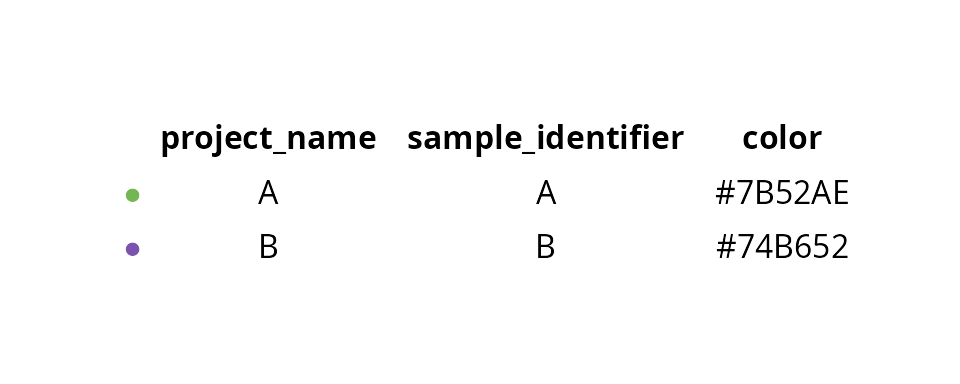
We set main parameters:
n_threads = 10L
cl = aquarius::create_parallel_instance(nthreads = n_threads)
num_threads = n_threads # Rtsne::Rtsne option

ndims = 20
Load dataset
We load the Seurat object:
sobj = readRDS(data_path)
sobj
## An object of class Seurat
## 28000 features across 817 samples within 1 assay
## Active assay: RNA (28000 features, 3000 variable features)
## 3 layers present: counts, data, scale.data
## 2 dimensional reductions calculated: RNA_pca, RNA_pca_20_tsneWhat is the content of metadata ?
summary(sobj@meta.data)## orig.ident nCount_RNA nFeature_RNA log_nCount_RNA score_macrophages
## A:817 Min. : 106 Min. : 92 Min. : 4.663 Min. :-1.3456
## 1st Qu.: 1965 1st Qu.: 924 1st Qu.: 7.583 1st Qu.:-0.8058
## Median : 5299 Median :1924 Median : 8.575 Median :-0.2087
## Mean : 7229 Mean :2105 Mean : 8.333 Mean :-0.1525
## 3rd Qu.:11002 3rd Qu.:3066 3rd Qu.: 9.306 3rd Qu.: 0.5406
## Max. :56790 Max. :7097 Max. :10.947 Max. : 1.3188
##
## score_tumor_cells cell_type Seurat.Phase cyclone.Phase
## Min. :-0.9899 macrophages:413 Length:817 Length:817
## 1st Qu.:-0.7875 tumor cells:404 Class :character Class :character
## Median :-0.3143 Mode :character Mode :character
## Mean :-0.1463
## 3rd Qu.: 0.3578
## Max. : 2.2130
##
## RNA_snn_res.0.5 seurat_clusters percent.mt percent.rb
## 0 :232 0 :232 Min. : 0.000 Min. : 0.000
## 1 :226 1 :226 1st Qu.: 2.866 1st Qu.: 2.475
## 2 :145 2 :145 Median : 4.624 Median : 6.631
## 3 : 82 3 : 82 Mean : 8.151 Mean : 7.383
## 4 : 52 4 : 52 3rd Qu.:10.995 3rd Qu.:10.369
## 5 : 50 5 : 50 Max. :49.735 Max. :42.983
## (Other): 30 (Other): 30
## doublets_consensus.class scDblFinder.class hybrid_score.class fail_qc
## Mode :logical Mode :logical Mode :logical Mode :logical
## FALSE:634 FALSE:668 FALSE:642 FALSE:563
## TRUE :66 TRUE :32 TRUE :58 TRUE :254
## NA's :117 NA's :117 NA's :117
##
##
## Filtering
We apply the quality control based filtering:
sobj = subset(sobj, fail_qc == FALSE)
sobj
## An object of class Seurat
## 28000 features across 563 samples within 1 assay
## Active assay: RNA (28000 features, 3000 variable features)
## 3 layers present: counts, data, scale.data
## 2 dimensional reductions calculated: RNA_pca, RNA_pca_20_tsneWe remove the columns related to quality control:
sobj$fail_qc = NULL
sobj$doublets_consensus.class = NULL
sobj$scDblFinder.class = NULL
sobj$hybrid_score.class = NULL

summary(sobj@meta.data)
## orig.ident nCount_RNA nFeature_RNA log_nCount_RNA score_macrophages
## A:563 Min. : 1014 Min. : 600 Min. : 6.922 Min. :-1.34565
## 1st Qu.: 2817 1st Qu.:1300 1st Qu.: 7.943 1st Qu.:-0.84341
## Median : 6340 Median :2411 Median : 8.755 Median : 0.01314
## Mean : 7893 Mean :2363 Mean : 8.661 Mean :-0.10095
## 3rd Qu.:11597 3rd Qu.:3144 3rd Qu.: 9.358 3rd Qu.: 0.63424
## Max. :37168 Max. :5858 Max. :10.523 Max. : 1.31880
##
## score_tumor_cells cell_type Seurat.Phase cyclone.Phase
## Min. :-0.9899 macrophages:307 Length:563 Length:563
## 1st Qu.:-0.8251 tumor cells:256 Class :character Class :character
## Median :-0.5903 Mode :character Mode :character
## Mean :-0.1723
## 3rd Qu.: 0.5180
## Max. : 2.2130
##
## RNA_snn_res.0.5 seurat_clusters percent.mt percent.rb
## 0 :198 0 :198 Min. : 0.09302 Min. : 0.1894
## 1 :158 1 :158 1st Qu.: 2.78933 1st Qu.: 3.7768
## 3 : 66 3 : 66 Median : 4.27119 Median : 7.2535
## 4 : 49 4 : 49 Mean : 6.61453 Mean : 7.3381
## 2 : 46 2 : 46 3rd Qu.: 9.99721 3rd Qu.:10.4101
## 5 : 17 5 : 17 Max. :19.95874 Max. :19.6207
## (Other): 29 (Other): 29Processing
In this section, we process the dataset to annotate cells and generate 2D projection.
Normalization
We normalize the count matrix and identity the most variable features, among the remaining cells.
sobj = Seurat::NormalizeData(sobj,
                             normalization.method = "LogNormalize",
                             assay = "RNA")

sobj = Seurat::FindVariableFeatures(sobj,
                                    assay = "RNA",
                                    nfeatures = 3000)
sobj
## An object of class Seurat
## 28000 features across 563 samples within 1 assay
## Active assay: RNA (28000 features, 3000 variable features)
## 3 layers present: counts, data, scale.data
## 2 dimensional reductions calculated: RNA_pca, RNA_pca_20_tsneProjection
We perform the PCA:
sobj = Seurat::ScaleData(sobj)
sobj = Seurat::RunPCA(sobj,
                      assay = "RNA",
                      reduction.name = "RNA_pca",
                      npcs = 100)

Seurat::ElbowPlot(sobj, ndims = 100, reduction = "RNA_pca")
We generate a tSNE and a UMAP with 20 principal components:
sobj = Seurat::RunTSNE(sobj,
                       reduction = "RNA_pca",
                       dims = 1:ndims,
                       seed.use = 1337L,
                       reduction.name = paste0("RNA_pca_", ndims, "_tsne"),
                       num_threads = num_threads)

sobj = Seurat::RunUMAP(sobj,
                       reduction = "RNA_pca",
                       dims = 1:ndims,
                       seed.use = 1337L,
                       reduction.name = paste0("RNA_pca_", ndims, "_umap"))
Annotation
Cell type
We annotate cells for cell type, with the new normalized expression matrix:
sobj = aquarius::cell_annot_custom(sobj,
                                   newname = "cell_type",
                                   markers = cell_markers,
                                   use_negative = TRUE,
                                   add_score = TRUE)

table(sobj$cell_type)
##
## macrophages tumor cells
## 308 255To justify cell type annotation, we can make a dotplot:
aquarius::plot_dotplot(sobj, assay = "RNA",
                       column_name = "cell_type",
                       markers = dotplot_markers,
                       nb_hline = 0) +
  ggplot2::scale_color_gradientn(colors = aquarius::palette_GrOrBl) +
  ggplot2::theme(legend.position = "right",
                 legend.box = "vertical",
                 legend.direction = "vertical",
                 axis.title = element_blank(),
                 axis.text = element_text(size = 15))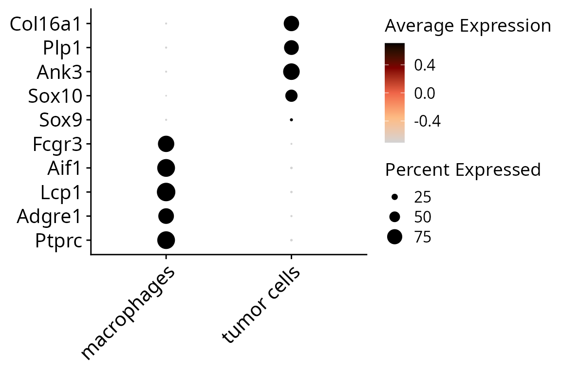
We can make a barplot to see the composition of each dataset, and visualize cell types on the projection.
df_proportion = as.data.frame(prop.table(table(sobj$orig.ident,
                                               sobj$cell_type)))
colnames(df_proportion) = c("orig.ident", "cell_type", "freq")

quantif = table(sobj$orig.ident) %>%
  as.data.frame.table() %>%
  `colnames<-`(c("orig.ident", "nb_cells"))

# Plot
plot_list = list()

plot_list[[2]] = aquarius::plot_barplot(df = df_proportion,
                                        x = "orig.ident",
                                        y = "freq",
                                        fill = "cell_type",
                                        position = ggplot2::position_fill()) +
  ggplot2::scale_fill_manual(name = "Cell type",
                             values = color_markers[levels(df_proportion$cell_type)],
                             breaks = levels(df_proportion$cell_type)) +
  ggplot2::geom_label(data = quantif, inherit.aes = FALSE,
                      aes(x = orig.ident, y = 1.05, label = nb_cells),
                      label.size = 0)

plot_list[[1]] = Seurat::DimPlot(sobj, group.by = "cell_type",
                                 reduction = paste0("RNA_pca_", ndims, "_tsne")) +
  ggplot2::scale_color_manual(values = unlist(color_markers),
                              breaks = names(color_markers)) +
  ggplot2::labs(title = sample_name,
                subtitle = paste0(ncol(sobj), " cells")) +
  Seurat::NoLegend() + Seurat::NoAxes() +
  ggplot2::theme(aspect.ratio = 1,
                 plot.title = element_text(hjust = 0.5),
                 plot.subtitle = element_text(hjust = 0.5))

patchwork::wrap_plots(plot_list, nrow = 1, widths = c(6, 1))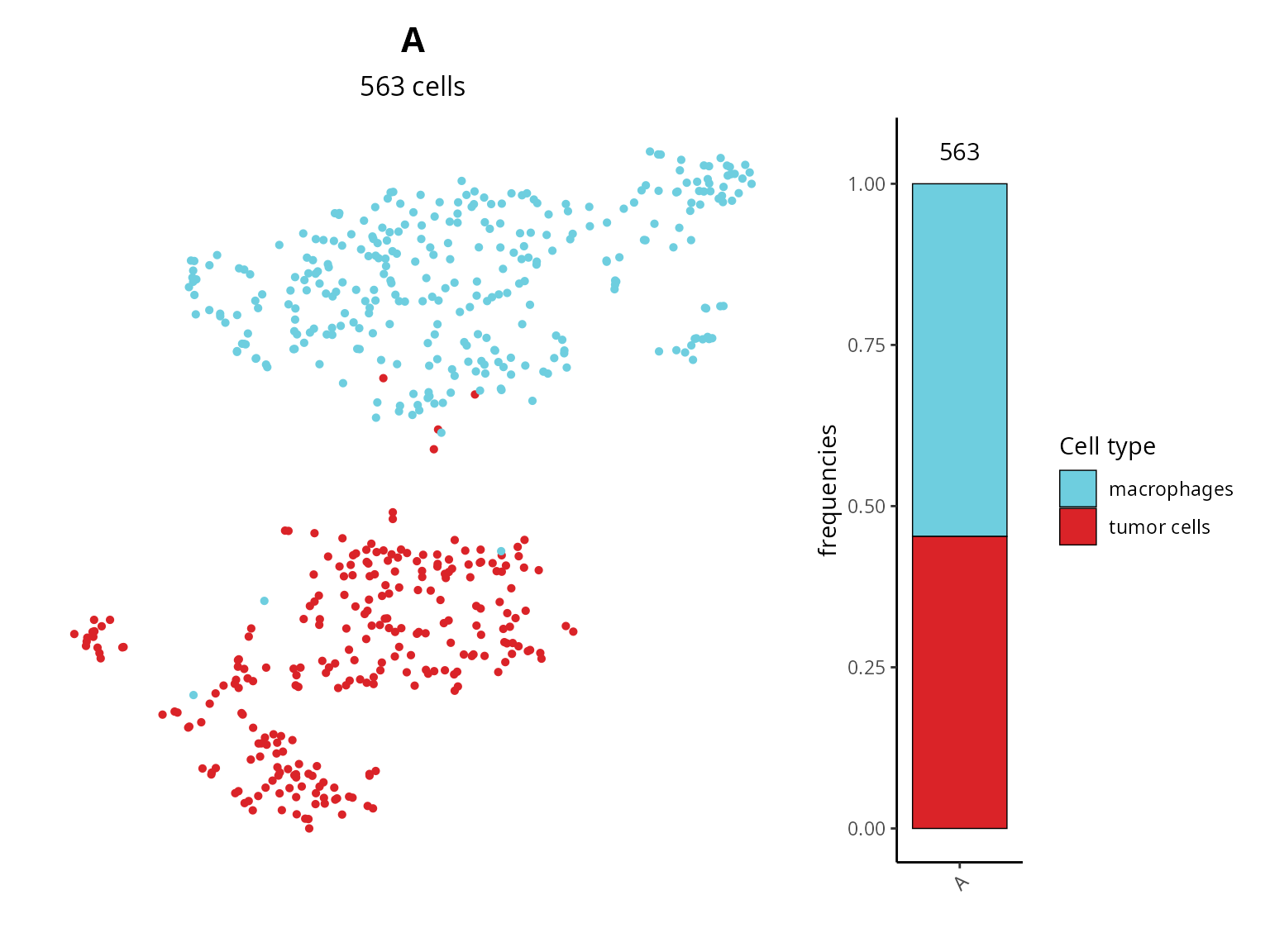
Cell cycle
We annotate cells for cell cycle phase:
cc_columns = aquarius::add_cell_cycle(sobj = sobj,
                                      assay = "RNA",
                                      species_rdx = "mm",
                                      BPPARAM = cl)@meta.data[, c("Seurat.Phase", "Phase")]

sobj$Seurat.Phase = cc_columns$Seurat.Phase
sobj$cyclone.Phase = cc_columns$Phase

table(sobj$Seurat.Phase, sobj$cyclone.Phase)
##
## G1 G2M S
## G1 329 10 2
## G2M 49 32 1
## S 136 3 1We visualize cell cycle on the projection:
plot_list = list()

plot_list[[2]] = Seurat::DimPlot(sobj, group.by = "Seurat.Phase",
                                 reduction = paste0("RNA_pca_", ndims, "_tsne")) +
  ggplot2::labs(title = "Cell Cycle Phase",
                subtitle = "Seurat.Phase") +
  Seurat::NoLegend() + Seurat::NoAxes() +
  ggplot2::theme(aspect.ratio = 1,
                 plot.title = element_text(hjust = 0.5),
                 plot.subtitle = element_text(hjust = 0.5))

plot_list[[1]] = Seurat::DimPlot(sobj, group.by = "cyclone.Phase",
                                 reduction = paste0("RNA_pca_", ndims, "_tsne")) +
  ggplot2::labs(title = "Cell Cycle Phase",
                subtitle = "cyclone.Phase") +
  Seurat::NoLegend() + Seurat::NoAxes() +
  ggplot2::theme(aspect.ratio = 1,
                 plot.title = element_text(hjust = 0.5),
                 plot.subtitle = element_text(hjust = 0.5))

patchwork::wrap_plots(plot_list, nrow = 1)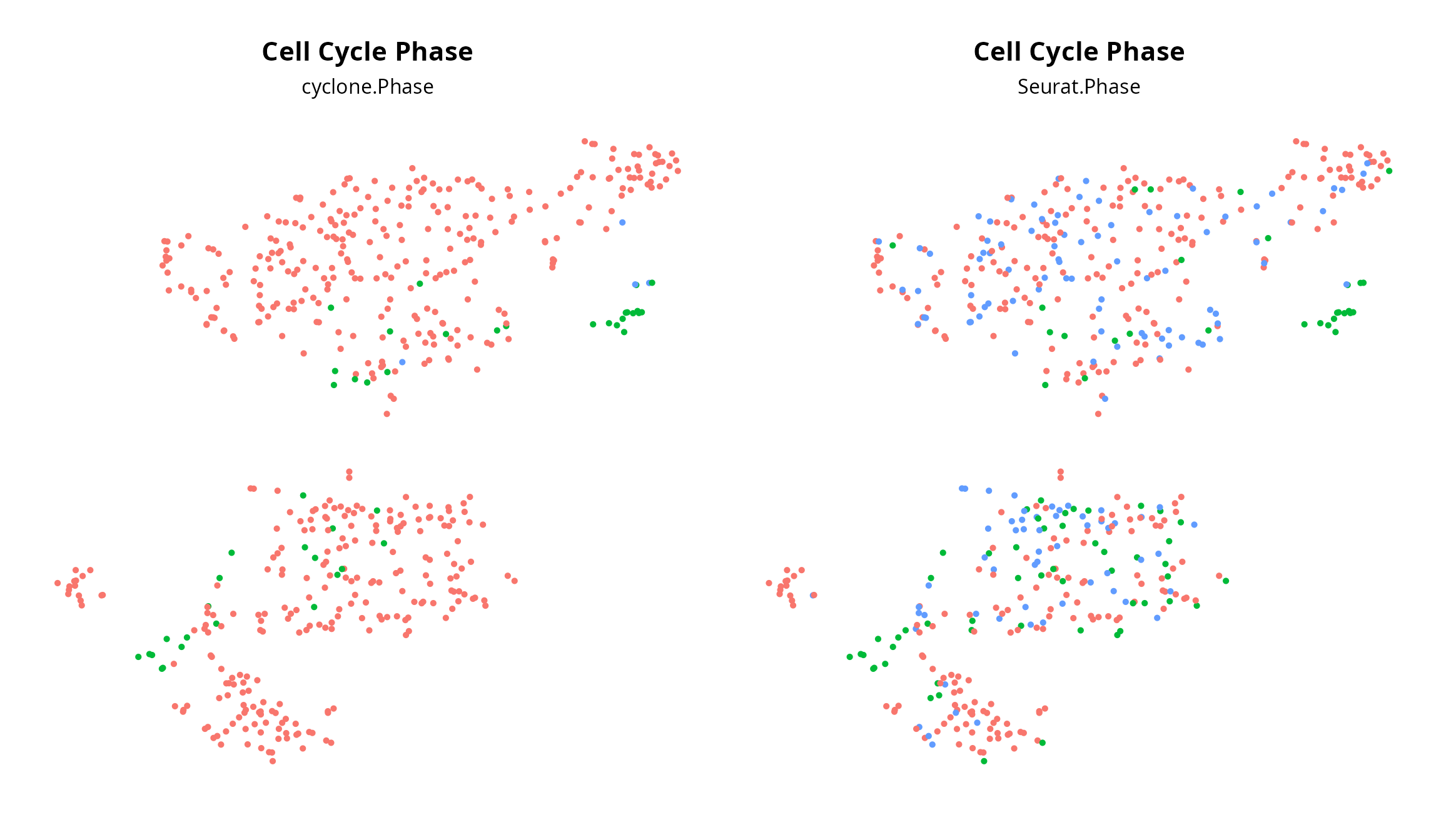
Clustering
We make a clustering:
sobj = Seurat::FindNeighbors(sobj, reduction = "RNA_pca", dims = c(1:ndims))
sobj = Seurat::FindClusters(sobj, resolution = 0.5)
## Modularity Optimizer version 1.3.0 by Ludo Waltman and Nees Jan van Eck
##
## Number of nodes: 563
## Number of edges: 17333
##
## Running Louvain algorithm...
## Maximum modularity in 10 random starts: 0.8140
## Number of communities: 6
## Elapsed time: 0 seconds
table(sobj$seurat_clusters)##
## 0 1 2 3 4 5
## 192 166 75 72 46 12Visualization
Quality metrics
We visualize the 4 quality-related metrics:
p1 = lapply(c("nFeature_RNA", "log_nCount_RNA",
              "percent.mt", "percent.rb"), FUN = function(one_metric) {
                p = Seurat::FeaturePlot(sobj, features = one_metric,
                                        reduction = paste0("RNA_pca_", ndims, "_tsne")) +
                  ggplot2::scale_color_gradientn(colors = aquarius::palette_GrOrBl) +
                  ggplot2::theme(aspect.ratio = 1) +
                  Seurat::NoAxes()
                return(p)
              })

p2 = lapply(c("nFeature_RNA", "log_nCount_RNA",
              "percent.mt", "percent.rb"), FUN = function(one_metric) {
                p = Seurat::FeaturePlot(sobj, features = one_metric,
                                        reduction = paste0("RNA_pca_", ndims, "_umap")) +
                  ggplot2::scale_color_gradientn(colors = aquarius::palette_GrOrBl) +
                  ggplot2::theme(aspect.ratio = 1) +
                  Seurat::NoAxes()
                return(p)
              })

patchwork::wrap_plots(unlist(list(p1, p2), recursive = FALSE), ncol = 4)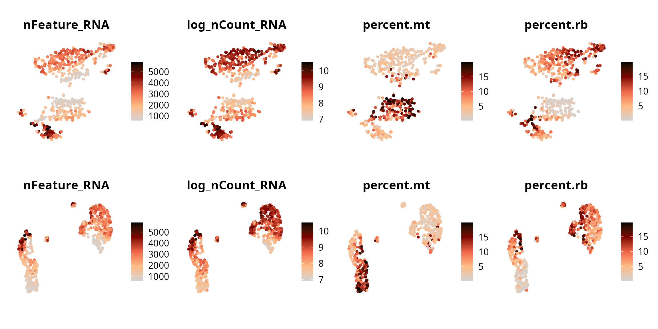
Cell type
We can visualize the cell type:
tsne = Seurat::DimPlot(sobj, group.by = "cell_type",
                       reduction = paste0("RNA_pca_", ndims, "_tsne"), cols = color_markers) +
  Seurat::NoAxes() + ggplot2::ggtitle("tSNE") +
  ggplot2::theme(aspect.ratio = 1,
                 plot.title = element_text(hjust = 0.5),
                 legend.position = "none")

umap = Seurat::DimPlot(sobj, group.by = "cell_type",
                       reduction = paste0("RNA_pca_", ndims, "_umap"), cols = color_markers) +
  Seurat::NoAxes() + ggplot2::ggtitle("UMAP") +
  ggplot2::theme(aspect.ratio = 1,
                 plot.title = element_text(hjust = 0.5))

tsne | umap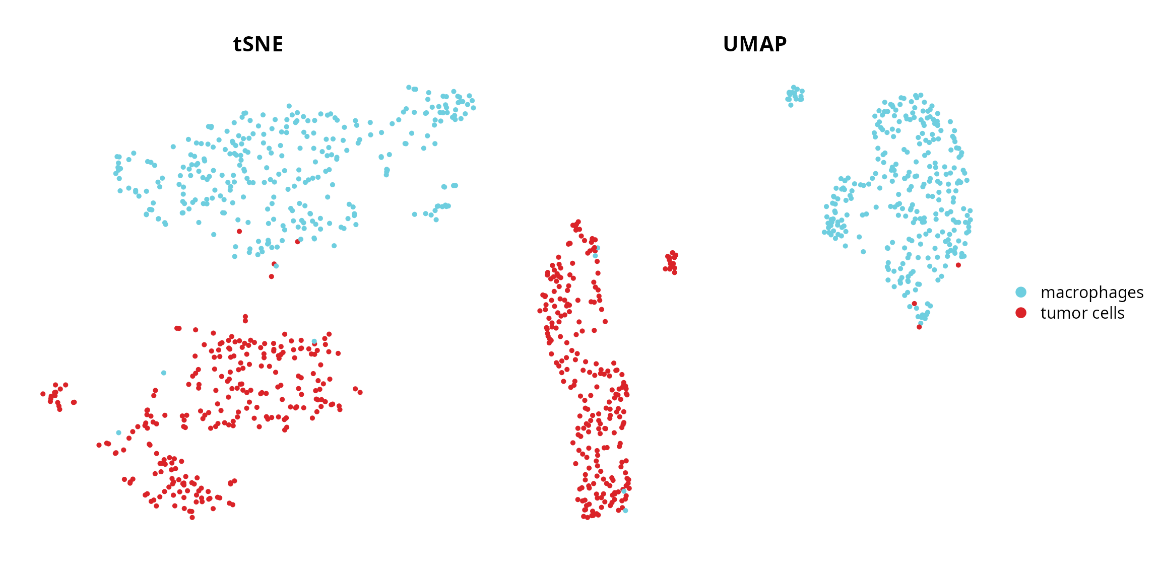
Cell cycle
We can visualize the cell cycle, from Seurat:
tsne = Seurat::DimPlot(sobj, group.by = "Seurat.Phase",
                       reduction = paste0("RNA_pca_", ndims, "_tsne")) +
  Seurat::NoAxes() + ggplot2::ggtitle("tSNE") +
  ggplot2::theme(aspect.ratio = 1,
                 plot.title = element_text(hjust = 0.5),
                 legend.position = "none")

umap = Seurat::DimPlot(sobj, group.by = "Seurat.Phase",
                       reduction = paste0("RNA_pca_", ndims, "_umap")) +
  Seurat::NoAxes() + ggplot2::ggtitle("UMAP") +
  ggplot2::theme(aspect.ratio = 1,
                 plot.title = element_text(hjust = 0.5))

tsne | umap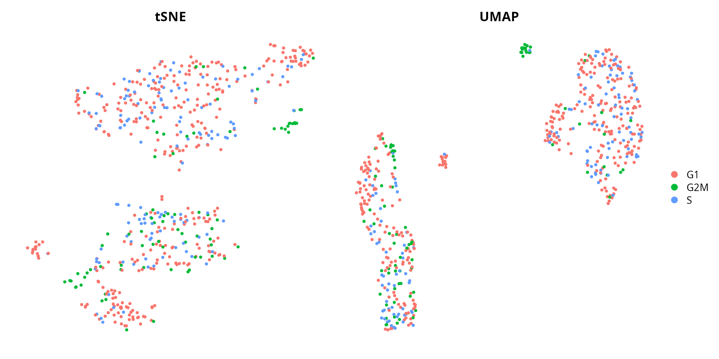
We can visualize the cell cycle, from cyclone:
tsne = Seurat::DimPlot(sobj, group.by = "cyclone.Phase",
                       reduction = paste0("RNA_pca_", ndims, "_tsne")) +
  Seurat::NoAxes() + ggplot2::ggtitle("tSNE") +
  ggplot2::theme(aspect.ratio = 1,
                 plot.title = element_text(hjust = 0.5),
                 legend.position = "none")

umap = Seurat::DimPlot(sobj, group.by = "cyclone.Phase",
                       reduction = paste0("RNA_pca_", ndims, "_umap")) +
  Seurat::NoAxes() + ggplot2::ggtitle("UMAP") +
  ggplot2::theme(aspect.ratio = 1,
                 plot.title = element_text(hjust = 0.5))

tsne | umap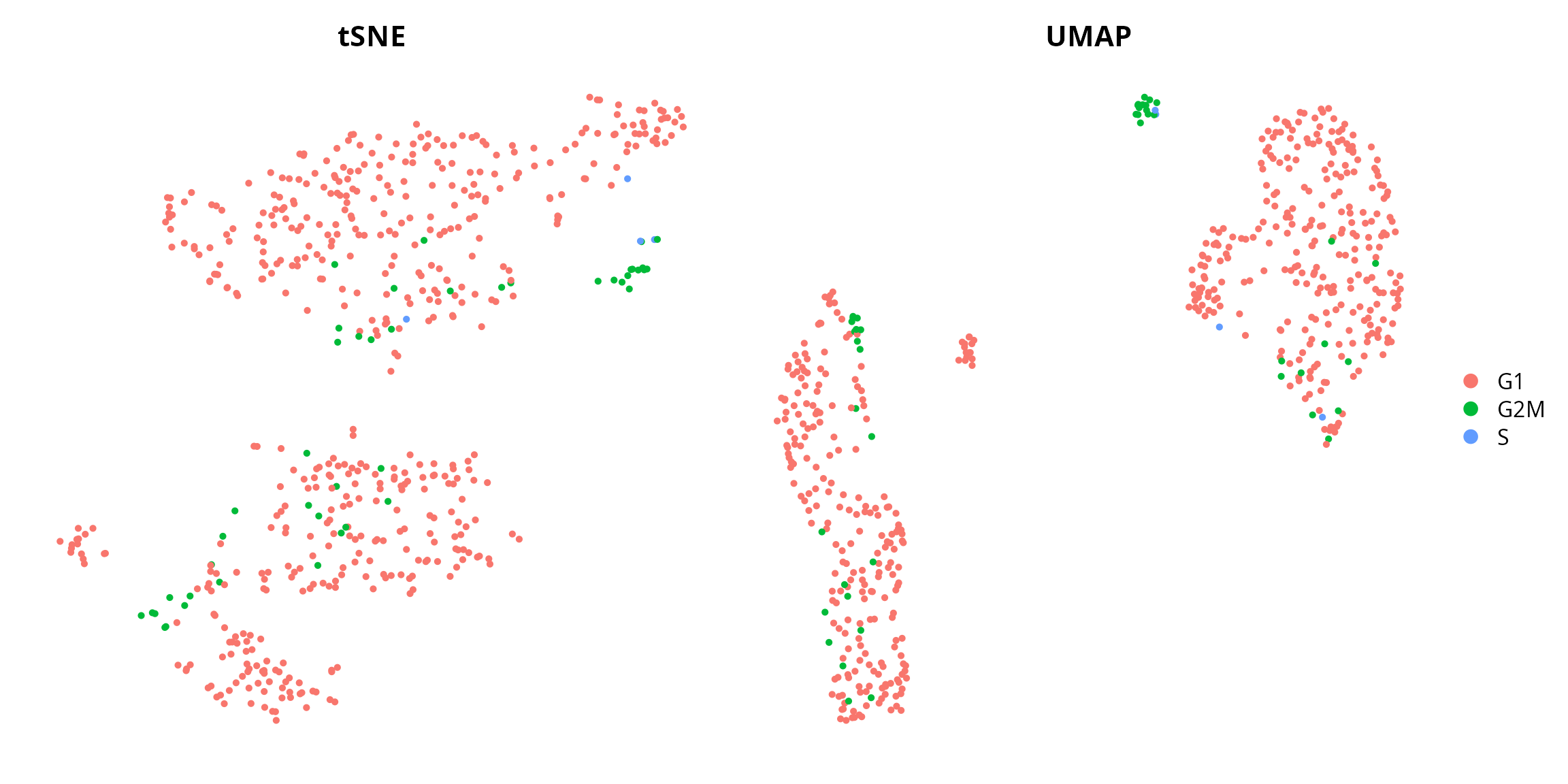
Clusters
We visualize the clustering:
tsne = Seurat::DimPlot(sobj, group.by = "seurat_clusters", label = TRUE,
                       reduction = paste0("RNA_pca_", ndims, "_tsne")) +
  Seurat::NoAxes() + ggplot2::ggtitle("tSNE") +
  ggplot2::theme(aspect.ratio = 1,
                 plot.title = element_text(hjust = 0.5),
                 legend.position = "none")

umap = Seurat::DimPlot(sobj, group.by = "seurat_clusters", label = TRUE,
                       reduction = paste0("RNA_pca_", ndims, "_umap")) +
  Seurat::NoAxes() + ggplot2::ggtitle("UMAP") +
  ggplot2::theme(aspect.ratio = 1,
                 plot.title = element_text(hjust = 0.5))

tsne | umap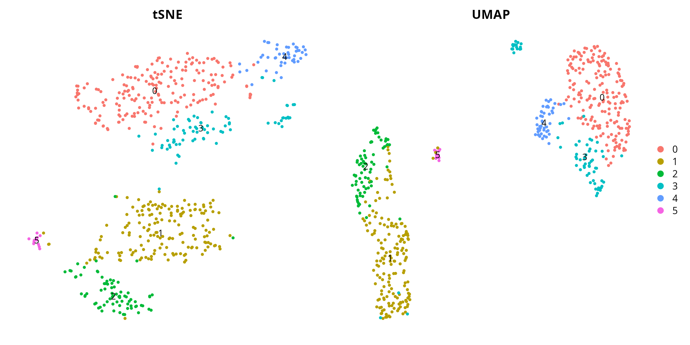
Gene expression
We visualize all cell types markers on the tSNE:
plot_list = lapply(dotplot_markers,
                   FUN = function(one_gene) {
                     p = Seurat::FeaturePlot(sobj, features = one_gene,
                                             reduction = paste0("RNA_pca_", ndims, "_tsne")) +
                       ggplot2::labs(title = one_gene) +
                       ggplot2::scale_color_gradientn(colors = aquarius::palette_GrOrBl) +
                       ggplot2::theme(aspect.ratio = 1,
                                      plot.subtitle = element_text(hjust = 0.5)) +
                       Seurat::NoAxes()
                     return(p)
                   })

patchwork::wrap_plots(plot_list)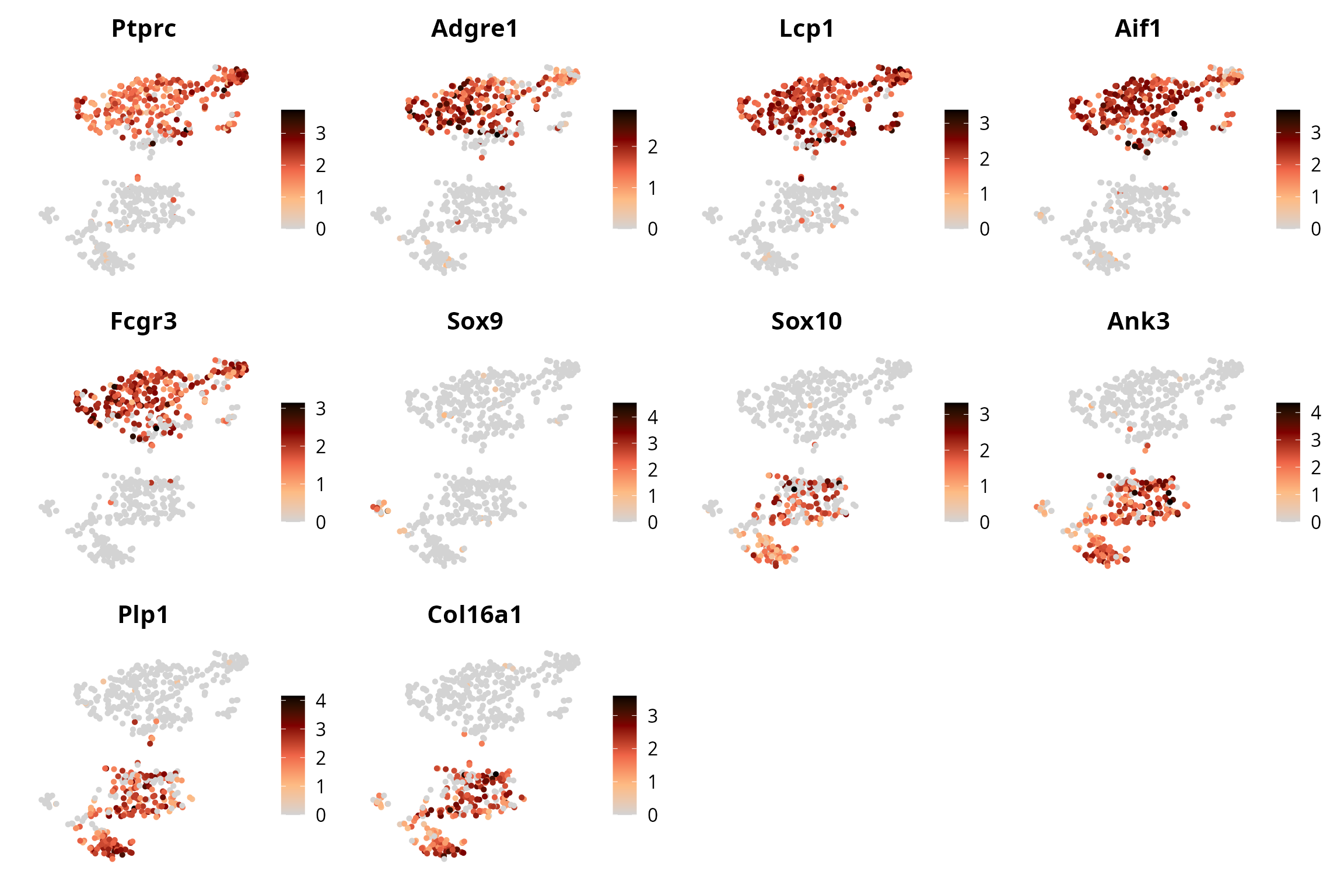
R Session
show
## R version 4.4.3 (2025-02-28)
## Platform: x86_64-pc-linux-gnu
## Running under: Ubuntu 24.10
##
## Matrix products: default
## BLAS:   /usr/lib/x86_64-linux-gnu/blas/libblas.so.3.12.0
## LAPACK: /usr/lib/x86_64-linux-gnu/lapack/liblapack.so.3.12.0
##
## locale:
##  [1] LC_CTYPE=en_US.UTF-8       LC_NUMERIC=C
##  [3] LC_TIME=fr_FR.UTF-8        LC_COLLATE=en_US.UTF-8
##  [5] LC_MONETARY=fr_FR.UTF-8    LC_MESSAGES=en_US.UTF-8
##  [7] LC_PAPER=fr_FR.UTF-8       LC_NAME=C
##  [9] LC_ADDRESS=C               LC_TELEPHONE=C
## [11] LC_MEASUREMENT=fr_FR.UTF-8 LC_IDENTIFICATION=C
##
## time zone: Europe/Paris
## tzcode source: system (glibc)
##
## attached base packages:
## [1] stats     graphics  grDevices utils     datasets  methods   base
##
## other attached packages:
## [1] future_1.40.0   ggplot2_3.5.2   patchwork_1.3.0 dplyr_1.1.4
##
## loaded via a namespace (and not attached):
##   [1] RcppAnnoy_0.0.22            splines_4.4.3
##   [3] later_1.4.2                 tibble_3.2.1
##   [5] polyclip_1.10-7             fastDummies_1.7.5
##   [7] lifecycle_1.0.4             edgeR_4.4.2
##   [9] doParallel_1.0.17           globals_0.17.0
##  [11] lattice_0.22-6              MASS_7.3-65
##  [13] magrittr_2.0.3              limma_3.62.2
##  [15] plotly_4.10.4               sass_0.4.10
##  [17] rmarkdown_2.29              jquerylib_0.1.4
##  [19] yaml_2.3.10                 metapod_1.14.0
##  [21] httpuv_1.6.16               Seurat_5.3.0
##  [23] sctransform_0.4.2           spam_2.11-1
##  [25] sp_2.2-0                    spatstat.sparse_3.1-0
##  [27] reticulate_1.42.0           cowplot_1.1.3
##  [29] pbapply_1.7-2               RColorBrewer_1.1-3
##  [31] abind_1.4-8                 zlibbioc_1.52.0
##  [33] Rtsne_0.17                  GenomicRanges_1.58.0
##  [35] purrr_1.0.4                 BiocGenerics_0.52.0
##  [37] circlize_0.4.16             GenomeInfoDbData_1.2.13
##  [39] IRanges_2.40.1              ggpattern_1.1.4
##  [41] S4Vectors_0.44.0            ggrepel_0.9.6
##  [43] irlba_2.3.5.1               listenv_0.9.1
##  [45] spatstat.utils_3.1-3        goftest_1.2-3
##  [47] RSpectra_0.16-2             spatstat.random_3.3-3
##  [49] dqrng_0.4.1                 fitdistrplus_1.2-2
##  [51] parallelly_1.43.0           pkgdown_2.1.2
##  [53] codetools_0.2-20            DelayedArray_0.32.0
##  [55] scuttle_1.16.0              tidyselect_1.2.1
##  [57] shape_1.4.6.1               UCSC.utils_1.2.0
##  [59] farver_2.1.2                ScaledMatrix_1.14.0
##  [61] matrixStats_1.5.0           stats4_4.4.3
##  [63] spatstat.explore_3.4-2      jsonlite_2.0.0
##  [65] GetoptLong_1.0.5            BiocNeighbors_2.0.1
##  [67] progressr_0.15.1            ggridges_0.5.6
##  [69] survival_3.8-3              iterators_1.0.14
##  [71] systemfonts_1.2.3           foreach_1.5.2
##  [73] tools_4.4.3                 ragg_1.4.0
##  [75] ica_1.0-3                   Rcpp_1.0.14
##  [77] glue_1.8.0                  gridExtra_2.3
##  [79] SparseArray_1.6.2           xfun_0.52
##  [81] MatrixGenerics_1.18.1       GenomeInfoDb_1.42.3
##  [83] withr_3.0.2                 fastmap_1.2.0
##  [85] bluster_1.16.0              digest_0.6.37
##  [87] rsvd_1.0.5                  R6_2.6.1
##  [89] mime_0.13                   textshaping_1.0.1
##  [91] colorspace_2.1-1            scattermore_1.2
##  [93] tensor_1.5                  spatstat.data_3.1-6
##  [95] tidyr_1.3.1                 generics_0.1.3
##  [97] data.table_1.17.0           httr_1.4.7
##  [99] htmlwidgets_1.6.4           S4Arrays_1.6.0
## [101] uwot_0.2.3                  pkgconfig_2.0.3
## [103] gtable_0.3.6                ComplexHeatmap_2.23.1
## [105] lmtest_0.9-40               SingleCellExperiment_1.28.1
## [107] XVector_0.46.0              htmltools_0.5.8.1
## [109] dotCall64_1.2               clue_0.3-66
## [111] SeuratObject_5.1.0          scales_1.4.0
## [113] Biobase_2.66.0              png_0.1-8
## [115] spatstat.univar_3.1-2       scran_1.34.0
## [117] knitr_1.50                  reshape2_1.4.4
## [119] rjson_0.2.23                aquarius_1.0.0
## [121] nlme_3.1-168                cachem_1.1.0
## [123] zoo_1.8-14                  GlobalOptions_0.1.2
## [125] stringr_1.5.1               KernSmooth_2.23-26
## [127] parallel_4.4.3              miniUI_0.1.2
## [129] desc_1.4.3                  pillar_1.10.2
## [131] grid_4.4.3                  vctrs_0.6.5
## [133] RANN_2.6.2                  promises_1.3.2
## [135] BiocSingular_1.22.0         beachmat_2.22.0
## [137] xtable_1.8-4                cluster_2.1.8.1
## [139] evaluate_1.0.3              locfit_1.5-9.12
## [141] cli_3.6.5                   compiler_4.4.3
## [143] rlang_1.1.6                 crayon_1.5.3
## [145] future.apply_1.11.3         labeling_0.4.3
## [147] plyr_1.8.9                  fs_1.6.6
## [149] stringi_1.8.7               viridisLite_0.4.2
## [151] deldir_2.0-4                BiocParallel_1.40.2
## [153] lazyeval_0.2.2              spatstat.geom_3.3-6
## [155] Matrix_1.7-3                RcppHNSW_0.6.0
## [157] statmod_1.5.0               shiny_1.10.0
## [159] SummarizedExperiment_1.36.0 ROCR_1.0-11
## [161] igraph_2.1.4                bslib_0.9.0