Analysis
Trajectory inference
2025-05-03
Source:vignettes/examples/3_analysis/1_trajectory.Rmd
1_trajectory.RmdThis notebook shows the use of these functions from
aquarius:
aquarius::traj_inferenceaquarius::traj_tingaaquarius::plot_label_dimplotaquarius::plot_selectoraquarius::find_features_order
The goal of this script is to merge perform trajectory inference and use related functions.
## [1] "/usr/lib/R/library"            "/usr/local/lib/R/site-library"
## [3] "/usr/lib/R/site-library"
Preparation
In this section, we set the global settings of the analysis. We will store data there:
out_dir = "."The input dataset is there:
save_name = "tumor_cells"
data_path = paste0(out_dir, "/../2_combined/", save_name, "_sobj.rds")

data_path
## [1] "./../2_combined/tumor_cells_sobj.rds"We define custom colors for each sample:
sample_info = data.frame(
  project_name = c("A", "B"),
  sample_identifier = c("A", "B"),
  color = c("#7B52AE", "#74B652"),
  row.names = c("A", "B"))

aquarius::plot_df(sample_info)
Load dataset
We load the dataset:
sobj = readRDS(data_path)

sobj
## An object of class Seurat
## 14361 features across 537 samples within 2 assays
## Active assay: RNA (12361 features, 2000 variable features)
## 3 layers present: scale.data, data, counts
## 1 other assay present: mnn.reconstructed
## 7 dimensional reductions calculated: RNA_pca, RNA_pca_51_tsne, RNA_pca_51_umap, mnn, mnn_51_umap, mnn_51_tsne, mnn_dmWe set the projection of interest:
name2D = "mnn_dm"Visualization
We visualize the expression levels of some genes on the diffusion map:
x_lim = range(sobj@reductions[[name2D]]@cell.embeddings[, 1])
y_lim = range(sobj@reductions[[name2D]]@cell.embeddings[, 2])

features_oi = c("nFeature_RNA", "Mbp", "Mgp", "Birc5")

plot_list = lapply(features_oi, FUN = function(one_gene) {
  p = Seurat::FeaturePlot(sobj, reduction = name2D,
                          pt.size = 0.25, order = TRUE,
                          features = one_gene) +
    ggplot2::lims(x = x_lim, y = y_lim) +
    Seurat::NoAxes() +
    ggplot2::scale_color_gradientn(colors = aquarius::palette_GrOrBl) +
    ggplot2::theme(aspect.ratio = 1)

  return(p)
})

patchwork::wrap_plots(plot_list, nrow = 1)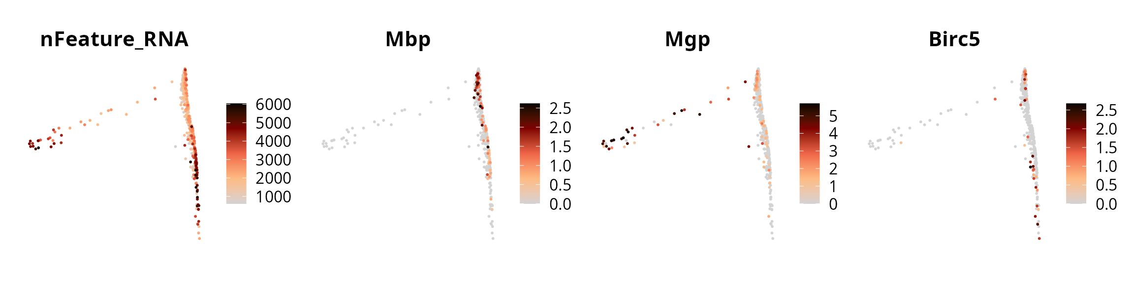
We visualize an interactive plot:
aquarius::plot_selector(sobj,
                        info_to_plot = "Mgp",
                        reduction = name2D)
Trajectory inference
Using TInGa
We set the root manually:
root_cell_id = "B_\"CCATCACTCGTGGCTG-1\""
sobj$is_root = colnames(sobj) == root_cell_id
sobj$cell_name = colnames(sobj)
root_plot = aquarius::plot_label_dimplot(sobj,
                                         reduction = name2D,
                                         col_by = "is_root",
                                         col_color = c("gray80", "red"),
                                         label_by = "cell_name",
                                         label_val = root_cell_id) +
  ggplot2::labs(title = "Root cell") +
  ggplot2::theme(plot.title = element_text(hjust = 0.5, face = "bold"),
                 aspect.ratio = 1) +
  Seurat::NoLegend() + Seurat::NoAxes()

sobj$is_root = NULL
sobj$cell_name = NULL

root_plot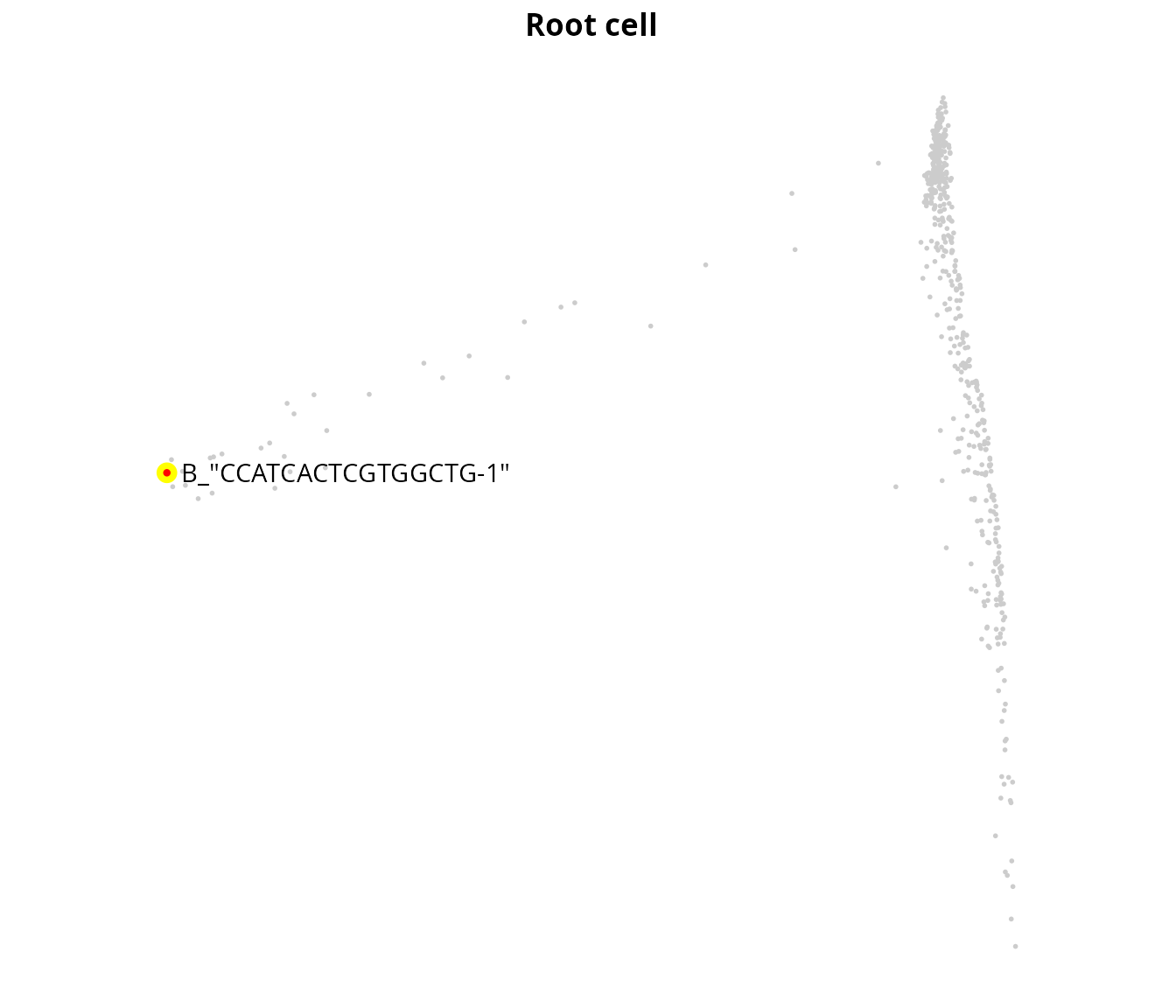
We perform trajectory inference:
traj_tinga = aquarius::traj_tinga(sobj,
                                  expression_assay = "RNA",
                                  expression_slot = "data",
                                  count_assay = "RNA",
                                  count_slot = "counts",
                                  dimred_name = "mnn",
                                  dimred_max_dim = 50,
                                  root_cell_id = root_cell_id)

class(traj_tinga)
## [1] "dynwrap::with_dimred" "dynwrap::with_trajectory"
## [3] "dynwrap::data_wrapper" "list"We add the pseudotime in the Seurat object:
sobj$pseudotime = traj_tinga$pseudotimeWe visualize the pseudotime using Seurat:
Seurat::FeaturePlot(sobj, features = "pseudotime",
                    reduction = name2D) +
  ggplot2::scale_color_gradientn(colors = viridis::viridis(n = 100)) +
  ggplot2::lims(x = x_lim, y = y_lim) +
  ggplot2::labs(title = "Pseudotime") +
  ggplot2::theme(aspect.ratio = 1,
                 plot.title = element_text(hjust = 0.5)) +
  Seurat::NoAxes()
We visualize the pseudotime using dynplot:
dynplot::plot_dimred(trajectory = traj_tinga,
                     label_milestones = FALSE,
                     plot_trajectory = TRUE,
                     dimred = sobj[[name2D]]@cell.embeddings,
                     color_cells = 'pseudotime',
                     color_trajectory = "none")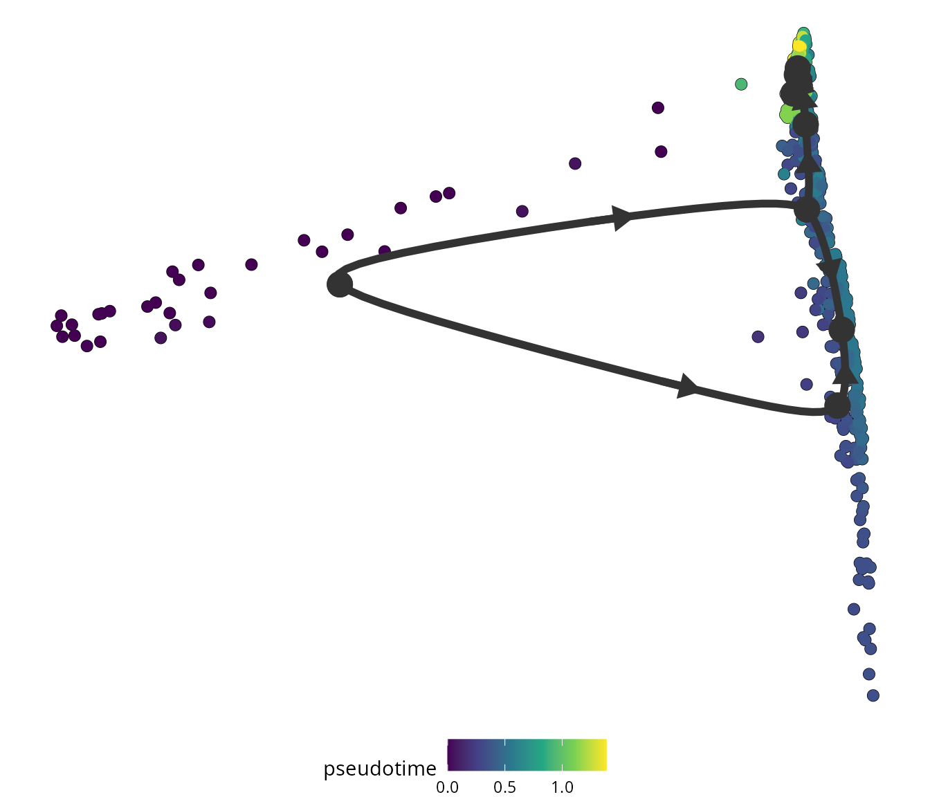
Using slingshot
We perform trajectory inference:
input_data = sobj@reductions[[name2D]]@cell.embeddings[, c(1:50)]

traj_slingshot = slingshot::slingshot(data = input_data,
                                      clusterLabels = sobj$seurat_clusters,
                                      start.clus   = sobj$seurat_clusters[root_cell_id])

class(traj_slingshot)
## [1] "PseudotimeOrdering"
## attr(,"package")
## [1] "TrajectoryUtils"Here is another way to do the same (eval = FALSE). But,
it is time consuming as it uses a software container.
traj_slingshot = aquarius::traj_inference(sobj,
                                          expression_assay = "RNA",
                                          expression_slot = "data",
                                          count_assay = "RNA",
                                          count_slot = "counts",
                                          dimred_name = name2D,
                                          dimred_max_dim = 50,
                                          root_cell_id = root_cell_id,
                                          ti_method = dynmethods::ti_slingshot())

class(traj_slingshot)
How many trajectories are available ?
head(slingshot::slingPseudotime(traj_slingshot))## Lineage1
## A_"AAACCCATCAAGTCGT-1" 0.5742917
## A_"AACACACCAGTAACAA-1" 0.6774816
## A_"AACGAAACAGTCACGC-1" 0.6615958
## A_"AACTTCTAGGGCCCTT-1" 0.6344614
## A_"AAGCGAGGTATCCCAA-1" 0.5974519
## A_"AAGTCGTAGTCACTAC-1" 0.6384976We add the associated pseudotime in the Seurat object:
sobj$pseudotime = slingshot::slingPseudotime(traj_slingshot)[, 1][colnames(sobj)]We visualize the pseudotime using Seurat:
Seurat::FeaturePlot(sobj, features = "pseudotime",
                    reduction = name2D) +
  ggplot2::scale_color_gradientn(colors = viridis::viridis(n = 100)) +
  ggplot2::lims(x = x_lim, y = y_lim) +
  ggplot2::labs(title = "Pseudotime") +
  ggplot2::theme(aspect.ratio = 1,
                 plot.title = element_text(hjust = 0.5)) +
  Seurat::NoAxes()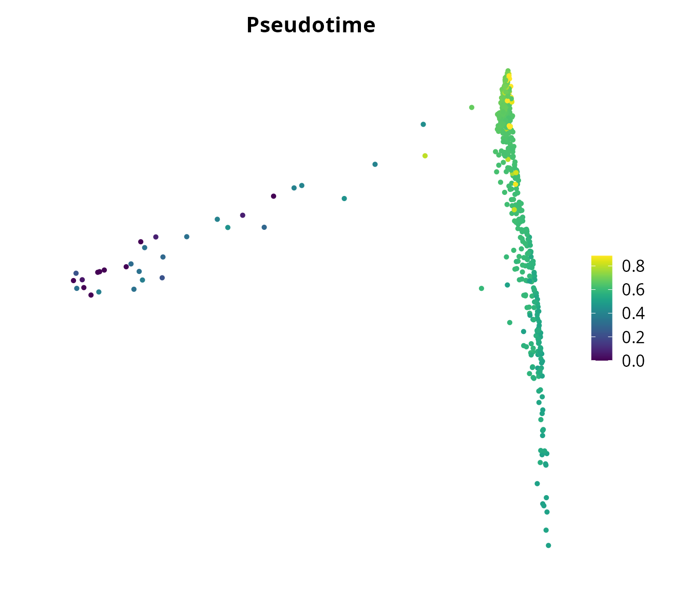
We visualize the pseudotime using the suggested method in
slingshot vignette.
# Reduction
rd = sobj[[name2D]]@cell.embeddings[, c(1:2)]

# Pseudotime
pdt = sobj$pseudotime

# Colors
colors = viridis::viridis(n = 100) # discrete
colors_plot = colors[cut(pdt, breaks = 100)]

# Plot
plot(rd,
     col = colors_plot,
     pch = 16,
     asp = 1)
lines(slingshot::SlingshotDataSet(traj_slingshot),
      lwd = 2,
      col = 'black')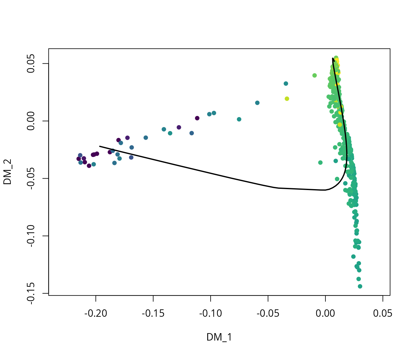
Heatmap
We identified genes of interest:
features = c("Mbp", "Dcn", "Birc5", "S100b", "Mgp")We define a matrix to make a heatmap from:
mat_expression = Seurat::GetAssayData(sobj, assay = "RNA", slot = "data")
mat_expression = mat_expression[features, ]
mat_expression = Matrix::t(mat_expression)
mat_expression = dynutils::scale_quantile(mat_expression) # between 0 and 1
mat_expression = Matrix::t(mat_expression)
mat_expression = Matrix::as.matrix(mat_expression)

dim(mat_expression)
## [1] 5 537We define custom colors:
list_colors = list()

list_colors[["expression"]] = aquarius::palette_BlWhRd

list_colors[["pseudotime"]] = circlize::colorRamp2(breaks = seq(min(sobj$pseudotime),
                                                                max(sobj$pseudotime),
                                                                length.out = 9),
                                                   colors = viridis::viridis(9))
We prepare the heatmap annotation:
ha_top = ComplexHeatmap::HeatmapAnnotation(
  pseudotime = sobj$pseudotime,
  annotation_legend_param = list(pseudotime = list(at = range(sobj$pseudotime),
                                                   labels = c("min", "max"))),
  col = list(pseudotime = list_colors[["pseudotime"]]))
Automatic order
We build a heatmap:
ht = ComplexHeatmap::Heatmap(
  mat_expression,
  # Expression colors
  col = list_colors[["expression"]],
  heatmap_legend_param = list(title = "expression", at = c(0, 1),
                              labels = c("low", "high")),
  # Annotation
  top_annotation = ha_top,
  # Cells order
  column_order = order(sobj$pseudotime),
  cluster_columns = FALSE,
  # Cells label
  show_column_names = FALSE,
  # Gene grouping
  cluster_rows = TRUE,
  show_row_dend = TRUE,
  # Gene labels
  row_labels = features,
  show_row_names = TRUE,
  row_names_gp = grid::gpar(fontsize = 12),
  # Visual aspect
  show_heatmap_legend = TRUE,
  border = TRUE,
  use_raster = FALSE)
We draw it:
ComplexHeatmap::draw(ht, # legend_grouping = "original",
                     merge_legend = TRUE,
                     heatmap_legend_side = "bottom",
                     annotation_legend_side = "bottom")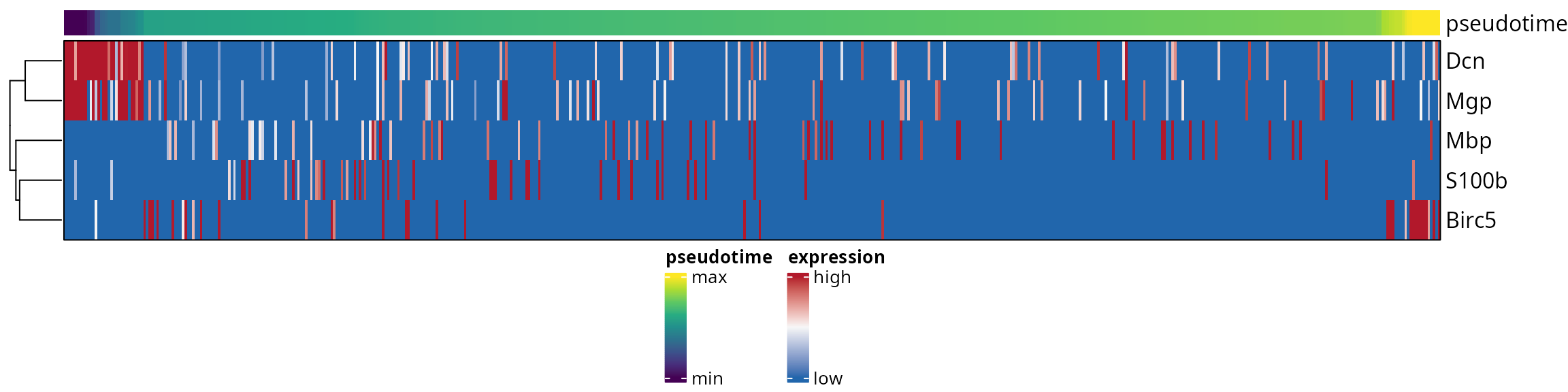
Pseudotime-consistent order
We identify an order to represent genes along pseudotime. First, we define a suited dataframe, containing the pseudotime and the genes of interest:
df_features = mat_expression %>%
  t() %>%
  as.data.frame.matrix()
df_features$pseudotime = sobj$pseudotime

head(df_features)
## Mbp Dcn Birc5 S100b Mgp pseudotime
## A_"AAACCCATCAAGTCGT-1" 0.0000000 0 0 1 0 0.5742917
## A_"AACACACCAGTAACAA-1" 0.0000000 0 0 0 0 0.6774816
## A_"AACGAAACAGTCACGC-1" 0.0000000 0 0 0 0 0.6615958
## A_"AACTTCTAGGGCCCTT-1" 0.0000000 0 0 0 0 0.6344614
## A_"AAGCGAGGTATCCCAA-1" 0.7775097 0 0 1 0 0.5974519
## A_"AAGTCGTAGTCACTAC-1" 1.0000000 0 0 0 0 0.6384976We use the aquarius::find_features_order function to
identify a beautiful order among genes:
features_order = aquarius::find_features_order(df_features)
features_order
## [1] "Mgp" "Dcn" "S100b" "Mbp" "Birc5"Now we can make the heatmap by forcing this ordering:
ht = ComplexHeatmap::Heatmap(
  mat_expression[features_order, ],   # <---- changed
  # Expression colors
  col = list_colors[["expression"]],
  heatmap_legend_param = list(title = "expression", at = c(0, 1),
                              labels = c("low", "high")),
  # Annotation
  top_annotation = ha_top,
  # Cells order
  column_order = order(sobj$pseudotime),
  cluster_columns = FALSE,
  # Cells label
  show_column_names = FALSE,
  # Gene grouping
  cluster_rows = FALSE,               # <---- changed
  show_row_dend = FALSE,              # <---- changed
  # Gene labels
  row_labels = features_order,        # <---- changed
  show_row_names = TRUE,
  row_names_gp = grid::gpar(fontsize = 12),
  # Visual aspect
  show_heatmap_legend = TRUE,
  border = TRUE,
  use_raster = FALSE)
We draw it:
ComplexHeatmap::draw(ht, # legend_grouping = "original",
                     merge_legend = TRUE,
                     heatmap_legend_side = "bottom",
                     annotation_legend_side = "bottom")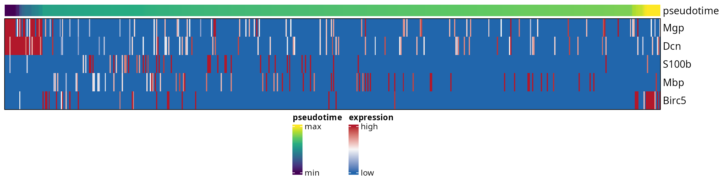
R Session
show
## R version 4.4.3 (2025-02-28)
## Platform: x86_64-pc-linux-gnu
## Running under: Ubuntu 24.10
##
## Matrix products: default
## BLAS:   /usr/lib/x86_64-linux-gnu/blas/libblas.so.3.12.0
## LAPACK: /usr/lib/x86_64-linux-gnu/lapack/liblapack.so.3.12.0
##
## locale:
##  [1] LC_CTYPE=en_US.UTF-8       LC_NUMERIC=C
##  [3] LC_TIME=fr_FR.UTF-8        LC_COLLATE=en_US.UTF-8
##  [5] LC_MONETARY=fr_FR.UTF-8    LC_MESSAGES=en_US.UTF-8
##  [7] LC_PAPER=fr_FR.UTF-8       LC_NAME=C
##  [9] LC_ADDRESS=C               LC_TELEPHONE=C
## [11] LC_MEASUREMENT=fr_FR.UTF-8 LC_IDENTIFICATION=C
##
## time zone: Europe/Paris
## tzcode source: system (glibc)
##
## attached base packages:
## [1] stats     graphics  grDevices utils     datasets  methods   base
##
## other attached packages:
## [1] dynutils_1.0.11 dynwrap_1.2.4   purrr_1.0.4     tidyr_1.3.1
## [5] ggplot2_3.5.2   patchwork_1.3.0 dplyr_1.1.4
##
## loaded via a namespace (and not attached):
##   [1] fs_1.6.6                    matrixStats_1.5.0
##   [3] spatstat.sparse_3.1-0       httr_1.4.7
##   [5] RColorBrewer_1.1-3          doParallel_1.0.17
##   [7] tools_4.4.3                 sctransform_0.4.2
##   [9] R6_2.6.1                    lazyeval_0.2.2
##  [11] uwot_0.2.3                  GetoptLong_1.0.5
##  [13] withr_3.0.2                 sp_2.2-0
##  [15] gridExtra_2.3               progressr_0.15.1
##  [17] cli_3.6.5                   Biobase_2.66.0
##  [19] textshaping_1.0.1           Cairo_1.6-2
##  [21] aquarius_1.0.0              spatstat.explore_3.4-2
##  [23] fastDummies_1.7.5           labeling_0.4.3
##  [25] sass_0.4.10                 Seurat_5.3.0
##  [27] spatstat.data_3.1-6         readr_2.1.5
##  [29] ggridges_0.5.6              pbapply_1.7-2
##  [31] pkgdown_2.1.2               slingshot_2.14.0
##  [33] systemfonts_1.2.3           parallelly_1.43.0
##  [35] GA_3.2.4                    TInGa_0.0.0.9000
##  [37] visNetwork_2.1.2            generics_0.1.3
##  [39] shape_1.4.6.1               ica_1.0-3
##  [41] spatstat.random_3.3-3       crosstalk_1.2.1
##  [43] Matrix_1.7-3                S4Vectors_0.44.0
##  [45] abind_1.4-8                 lifecycle_1.0.4
##  [47] yaml_2.3.10                 SummarizedExperiment_1.36.0
##  [49] SparseArray_1.6.2           Rtsne_0.17
##  [51] grid_4.4.3                  promises_1.3.2
##  [53] crayon_1.5.3                miniUI_0.1.2
##  [55] lattice_0.22-6              cowplot_1.1.3
##  [57] dynfeature_1.0.1            pillar_1.10.2
##  [59] knitr_1.50                  ComplexHeatmap_2.23.1
##  [61] GenomicRanges_1.58.0        rjson_0.2.23
##  [63] future.apply_1.11.3         codetools_0.2-20
##  [65] glue_1.8.0                  spatstat.univar_3.1-2
##  [67] data.table_1.17.0           remotes_2.5.0
##  [69] dynparam_1.0.2              vctrs_0.6.5
##  [71] png_0.1-8                   spam_2.11-1
##  [73] testthat_3.2.3              gtable_0.3.6
##  [75] assertthat_0.2.1            cachem_1.1.0
##  [77] xfun_0.52                   princurve_2.1.6
##  [79] S4Arrays_1.6.0              mime_0.13
##  [81] tidygraph_1.3.1             survival_3.8-3
##  [83] randomForestSRC_3.3.3       SingleCellExperiment_1.28.1
##  [85] iterators_1.0.14            DiagrammeR_1.0.11
##  [87] fitdistrplus_1.2-2          ROCR_1.0-11
##  [89] nlme_3.1-168                gng_0.1.0
##  [91] RcppAnnoy_0.0.22            GenomeInfoDb_1.42.3
##  [93] data.tree_1.1.0             bslib_0.9.0
##  [95] dyneval_0.9.9               irlba_2.3.5.1
##  [97] KernSmooth_2.23-26          colorspace_2.1-1
##  [99] BiocGenerics_0.52.0         carrier_0.1.1
## [101] tidyselect_1.2.1            processx_3.8.6
## [103] proxyC_0.5.2                compiler_4.4.3
## [105] desc_1.4.3                  DelayedArray_0.32.0
## [107] plotly_4.10.4               scales_1.4.0
## [109] lmtest_0.9-40               stringr_1.5.1
## [111] digest_0.6.37               goftest_1.2-3
## [113] spatstat.utils_3.1-3        rmarkdown_2.29
## [115] XVector_0.46.0              htmltools_0.5.8.1
## [117] pkgconfig_2.0.3             sparseMatrixStats_1.18.0
## [119] MatrixGenerics_1.18.1       fastmap_1.2.0
## [121] rlang_1.1.6                 GlobalOptions_0.1.2
## [123] htmlwidgets_1.6.4           UCSC.utils_1.2.0
## [125] DelayedMatrixStats_1.28.1   shiny_1.10.0
## [127] farver_2.1.2                jquerylib_0.1.4
## [129] zoo_1.8-14                  jsonlite_2.0.0
## [131] BiocParallel_1.40.2         magrittr_2.0.3
## [133] GenomeInfoDbData_1.2.13     dotCall64_1.2
## [135] dyndimred_1.0.4             Rcpp_1.0.14
## [137] viridis_0.6.5               reticulate_1.42.0
## [139] TrajectoryUtils_1.14.0      stringi_1.8.7
## [141] ggraph_2.2.1                brio_1.1.5
## [143] zlibbioc_1.52.0             MASS_7.3-65
## [145] dynplot_1.1.2               plyr_1.8.9
## [147] parallel_4.4.3              listenv_0.9.1
## [149] ggrepel_0.9.6               deldir_2.0-4
## [151] graphlayouts_1.2.2          splines_4.4.3
## [153] tensor_1.5                  hms_1.1.3
## [155] circlize_0.4.16             ps_1.9.1
## [157] igraph_2.1.4                ranger_0.17.0
## [159] spatstat.geom_3.3-6         babelwhale_1.2.0
## [161] RcppHNSW_0.6.0              reshape2_1.4.4
## [163] stats4_4.4.3                evaluate_1.0.3
## [165] SeuratObject_5.1.0          tzdb_0.5.0
## [167] foreach_1.5.2               tweenr_2.0.3
## [169] httpuv_1.6.16               RANN_2.6.2
## [171] polyclip_1.10-7             future_1.40.0
## [173] clue_0.3-66                 scattermore_1.2
## [175] lmds_0.1.0                  ggforce_0.4.2
## [177] xtable_1.8-4                RSpectra_0.16-2
## [179] later_1.4.2                 viridisLite_0.4.2
## [181] ragg_1.4.0                  tibble_3.2.1
## [183] memoise_2.0.1               IRanges_2.40.1
## [185] cluster_2.1.8.1             globals_0.17.0