Analysis
Gene analysis
2025-05-03
Source:vignettes/examples/3_analysis/2_gene_analysis.Rmd
2_gene_analysis.RmdThis notebook shows the use of these functions from
aquarius:
aquarius::get_gene_setsaquarius::gg_color_hueaquarius::find_features_orderaquarius::run_enrichraquarius::run_gseaaquarius::plot_dfaquarius::plot_alluvialaquarius::plot_piechart_subpopulationaquarius::plot_red_and_blueaquarius::plot_pctaquarius::plot_violinaquarius::plot_wordcloudaquarius::plot_gsea_barplotaquarius::plot_gsea_curve
The goal of this script is to make:
- differential expression analysis
- over-representation analysis
- gene set enrichment analysis
and to illustrate the use of aquarius functions, mostly
related to visualization.
## [1] "/usr/lib/R/library"            "/usr/local/lib/R/site-library"
## [3] "/usr/lib/R/site-library"
Preparation
In this section, we set the global settings of the analysis. Data are stored there:
out_dir = "."The input dataset is there:
save_name = "combined"
data_path = paste0(out_dir, "/../2_combined/", save_name, "_sobj.rds")

data_path
## [1] "./../2_combined/combined_sobj.rds"Here are custom colors for each cell type:
color_markers = c("macrophages" = "#6ECEDF",
                  "tumor cells" = "#DA2328")
We define custom colors for each sample:
sample_info = data.frame(
  project_name = c("A", "B"),
  sample_identifier = c("A", "B"),
  color = c("#7B52AE", "#74B652"),
  row.names = c("A", "B"))

aquarius::plot_df(sample_info)
We set main parameters:
n_threads = 5L # AUCell::AUCell_buildRankingsLoad dataset
We load the dataset:
sobj = readRDS(data_path)

sobj
## An object of class Seurat
## 13774 features across 1108 samples within 1 assay
## Active assay: RNA (13774 features, 2000 variable features)
## 3 layers present: scale.data, data, counts
## 6 dimensional reductions calculated: RNA_pca, RNA_pca_48_tsne, RNA_pca_48_umap, harmony, harmony_48_umap, harmony_48_tsneWe set the projection of interest:
name2D = "harmony_48_tsne"Visualization
We represent the 4 quality metrics:
features = c("percent.mt", "percent.rb", "log_nCount_RNA", "nFeature_RNA")

plot_list = lapply(features, FUN = function(one_feature) {
  p = Seurat::FeaturePlot(sobj, reduction = name2D,
                          pt.size = 0.25,
                          features = one_feature) +
    ggplot2::scale_color_gradientn(colors = aquarius::palette_GrOrBl) +
    Seurat::NoAxes() +
    ggplot2::theme(aspect.ratio = 1)

  return(p)
})

patchwork::wrap_plots(plot_list, nrow = 1)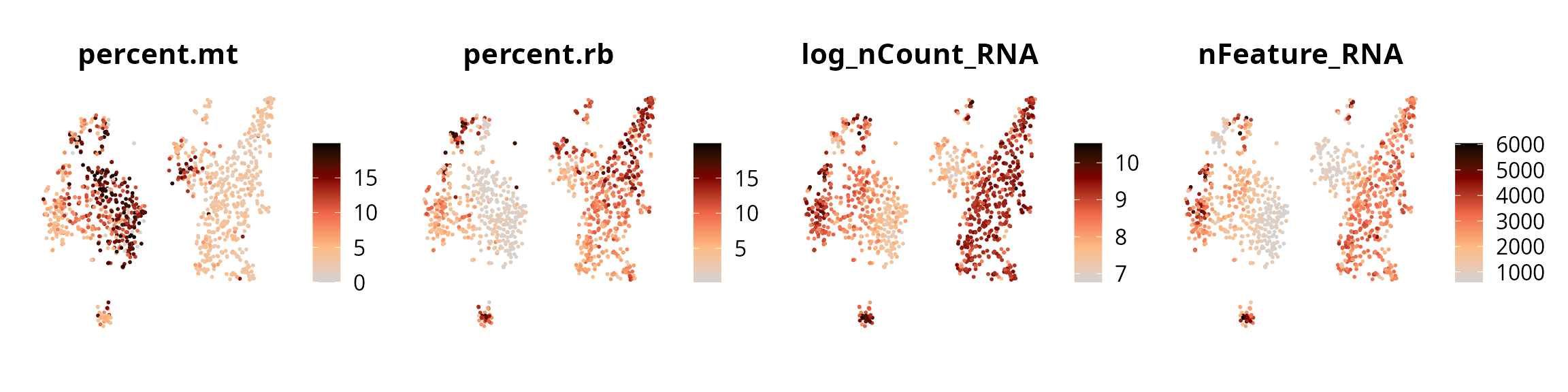
Clusters
We visualize the clusters:
Seurat::DimPlot(sobj, reduction = name2D,
                group.by = "seurat_clusters",
                label = TRUE) +
  Seurat::NoLegend() +
  Seurat::NoAxes() +
  ggplot2::theme(aspect.ratio = 1)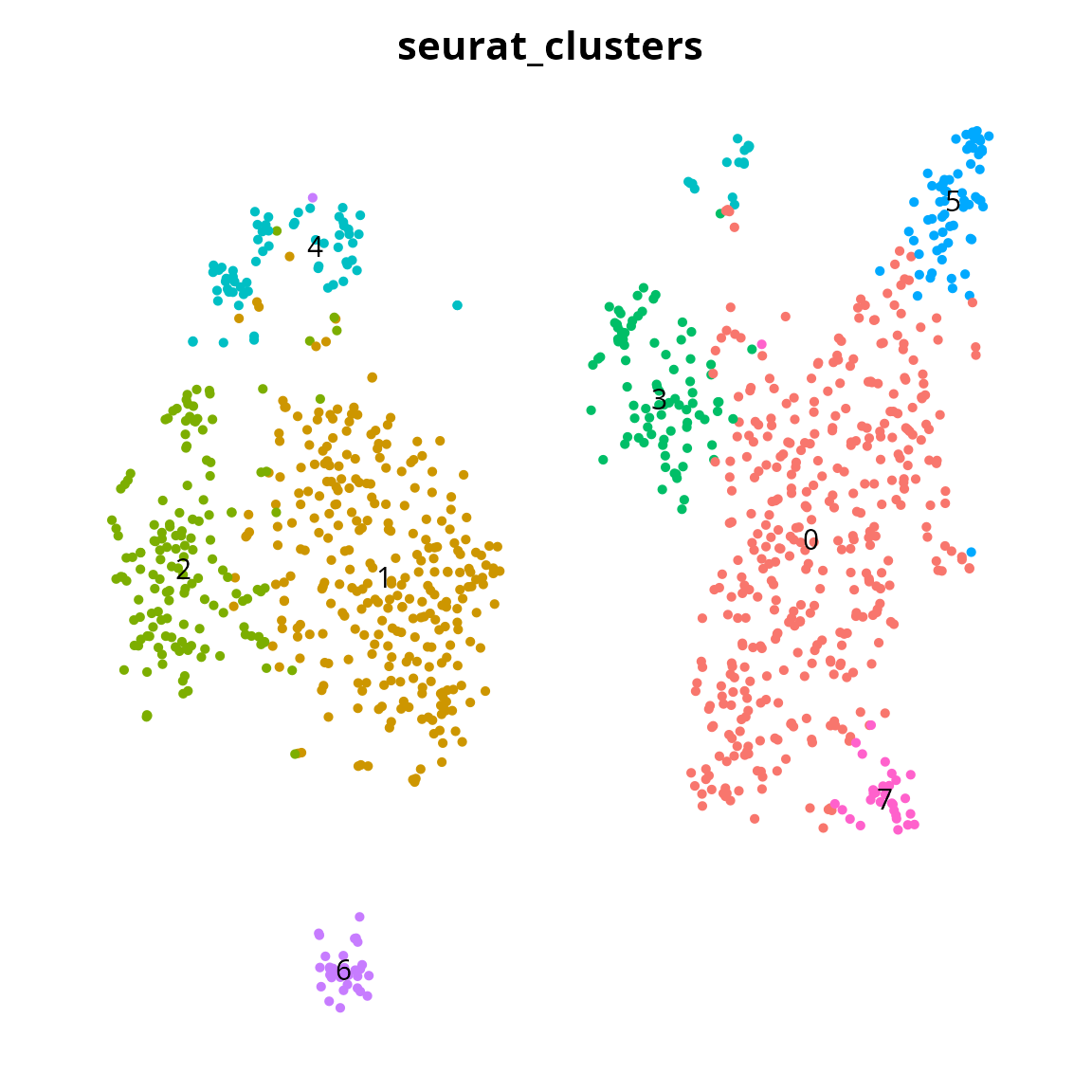
Cell type
We visualize the cell type annotation:
Seurat::DimPlot(sobj, reduction = name2D,
                group.by = "cell_type",
                cols = color_markers) +
  Seurat::NoAxes() +
  ggplot2::theme(aspect.ratio = 1)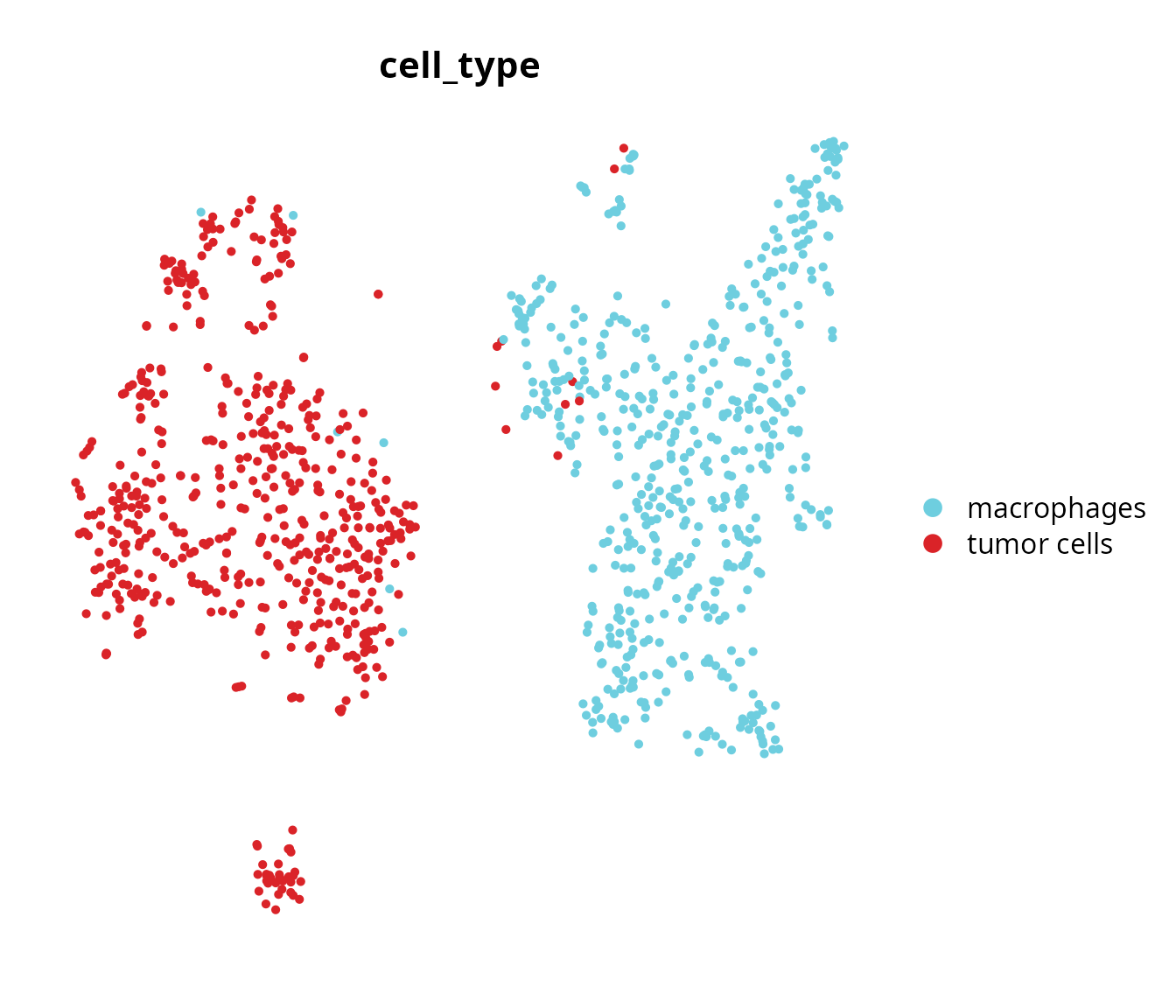
Sample of origin
We visualize the cells colored according to their sample of origin.
Seurat::DimPlot(sobj, reduction = name2D,
                group.by = "orig.ident") +
  ggplot2::scale_color_manual(values = sample_info$color,
                              breaks = sample_info$project_name) +
  Seurat::NoAxes() +
  ggplot2::theme(aspect.ratio = 1)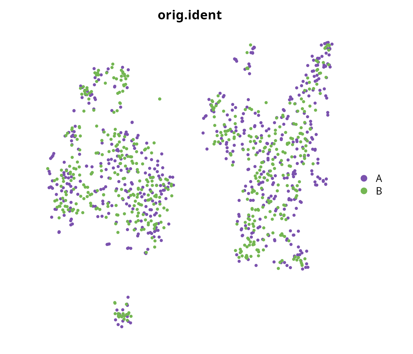
Analysis
The results will be stored in the list_results
object:
list_results = list()We get gene name and gene ID correspondence:
gene_corresp = sobj@assays[["RNA"]]@meta.data[, c("gene_name", "Ensembl_ID")] %>%
  `colnames<-`(c("NAME", "ID")) %>%
  dplyr::mutate(ID = as.character(ID))
rownames(gene_corresp) = gene_corresp$ID

head(gene_corresp)
## NAME ID
## ENSMUSG00000051951 Xkr4 ENSMUSG00000051951
## ENSMUSG00000033845 Mrpl15 ENSMUSG00000033845
## ENSMUSG00000025903 Lypla1 ENSMUSG00000025903
## ENSMUSG00000033813 Tcea1 ENSMUSG00000033813
## ENSMUSG00000033793 Atp6v1h ENSMUSG00000033793
## ENSMUSG00000025907 Rb1cc1 ENSMUSG00000025907We load gene sets from MSigDB:
gene_sets = aquarius::get_gene_sets(
  species = "Mus musculus",
  gs_collection = c("H", "C2", "C5"),
  gs_subcollection = c("", "GO:BP", "GO:MF", "GO:CC", "CP:KEGG", "CP:WIKIPATHWAYS",
                       "CP:REACTOME", "CP:PID"))

summary(gene_sets)
## gene_symbol ncbi_gene ensembl_gene db_gene_symbol
## Length:973643 Min. : 11298 Length:973643 Length:973643
## Class :character 1st Qu.: 16846 Class :character Class :character
## Mode :character Median : 27966 Mode :character Mode :character
## Mean : 659286
## 3rd Qu.: 99371
## Max. :115489950
## NA's :93
## db_ncbi_gene db_ensembl_gene source_gene gs_id
## Length:973643 Length:973643 Length:973643 Length:973643
## Class :character Class :character Class :character Class :character
## Mode :character Mode :character Mode :character Mode :character
##
##
##
##
## gs_name gs_collection gs_subcollection gs_collection_name
## Length:973643 Length:973643 Length:973643 Length:973643
## Class :character Class :character Class :character Class :character
## Mode :character Mode :character Mode :character Mode :character
##
##
##
##
## gs_description gs_source_species gs_pmid gs_geoid
## Length:973643 Length:973643 Length:973643 Length:973643
## Class :character Class :character Class :character Class :character
## Mode :character Mode :character Mode :character Mode :character
##
##
##
##
## gs_exact_source gs_url db_version db_target_species
## Length:973643 Length:973643 Length:973643 Length:973643
## Class :character Class :character Class :character Class :character
## Mode :character Mode :character Mode :character Mode :character
##
##
##
##
## ortholog_taxon_id ortholog_sources num_ortholog_sources
## Min. :10090 Length:973643 Min. : 3.00
## 1st Qu.:10090 Class :character 1st Qu.:11.00
## Median :10090 Mode :character Median :12.00
## Mean :10090 Mean :10.93
## 3rd Qu.:10090 3rd Qu.:12.00
## Max. :10090 Max. :12.00
## Select groups of interest
Here, we show the code to set the groups of interest to compare:
- a cluster and some/all others
- two (groups of) samples
- two (groups of) cell types
1. Cluster heterogeneity
We want to investigate the cluster heterogeneity among macrophages.
Cluster annotation
First, we need to identify the clusters corresponding to this cell population. We smooth the single-cell level cell type annotation over clusters:
We summarize major cell type by cluster:
sobj$cell_type = factor(sobj$cell_type,
                        levels = names(color_markers))

cell_type_clusters = sobj@meta.data[, c("cell_type", "seurat_clusters")] %>%
  table() %>%
  prop.table(., margin = 2) %>%
  apply(., 2, which.max)
cell_type_clusters = setNames(levels(sobj$cell_type)[cell_type_clusters],
                              nm = names(cell_type_clusters))

cell_type_clusters
## 0 1 2 3 4
## "macrophages" "tumor cells" "tumor cells" "macrophages" "tumor cells"
## 5 6 7
## "macrophages" "tumor cells" "macrophages"We define cluster type:
sobj$cluster_type = setNames(nm = colnames(sobj),
                             cell_type_clusters[sobj$seurat_clusters])
sobj$cluster_type = factor(sobj$cluster_type,
                           levels = levels(sobj$cell_type)) %>%
  droplevels()
We visualize the changes between cell type annotation and cluster annotation:
aquarius::plot_alluvial(sobj@meta.data,
                        column1 = "cell_type",
                        column2 = "cluster_type",
                        colors = color_markers) +
  ggplot2::guides(fill = ggplot2::guide_legend(override.aes = list(size = 5),
                                               ncol = 1))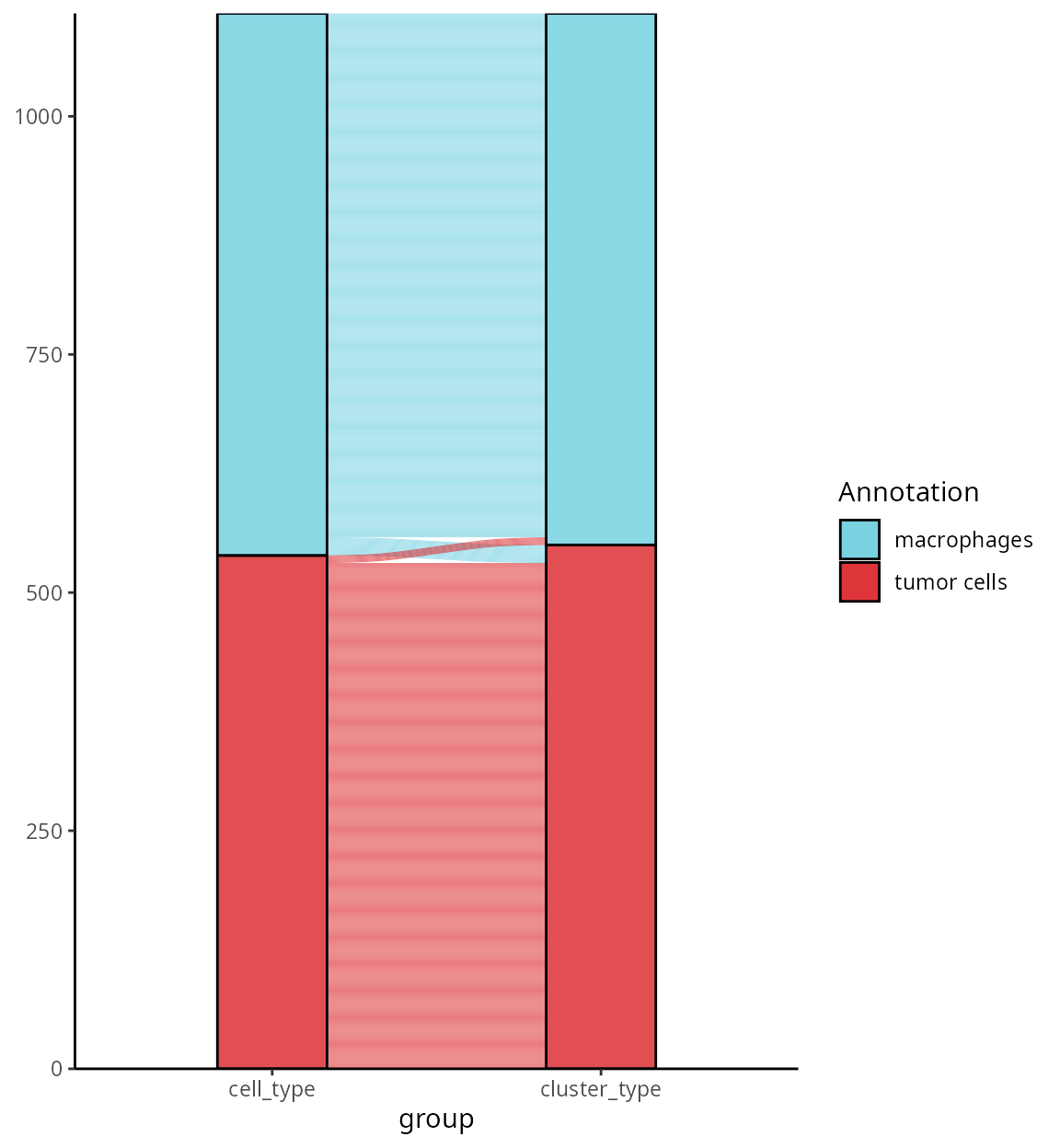
We compare cell type annotation and cluster annotation:
p1 = Seurat::DimPlot(sobj, group.by = "cell_type",
                     reduction = name2D, cols = color_markers) +
  ggplot2::labs(title = "Cell type") +
  Seurat::NoAxes() + Seurat::NoLegend() +
  ggplot2::theme(aspect.ratio = 1,
                 plot.title = element_text(hjust = 0.5))

p2 = Seurat::DimPlot(sobj, group.by = "cluster_type",
                     reduction = name2D, cols = color_markers) +
  ggplot2::labs(title = "Cluster type") +
  Seurat::NoAxes() +
  ggplot2::theme(aspect.ratio = 1,
                 plot.title = element_text(hjust = 0.5))

patchwork::wrap_plots(p1, p2)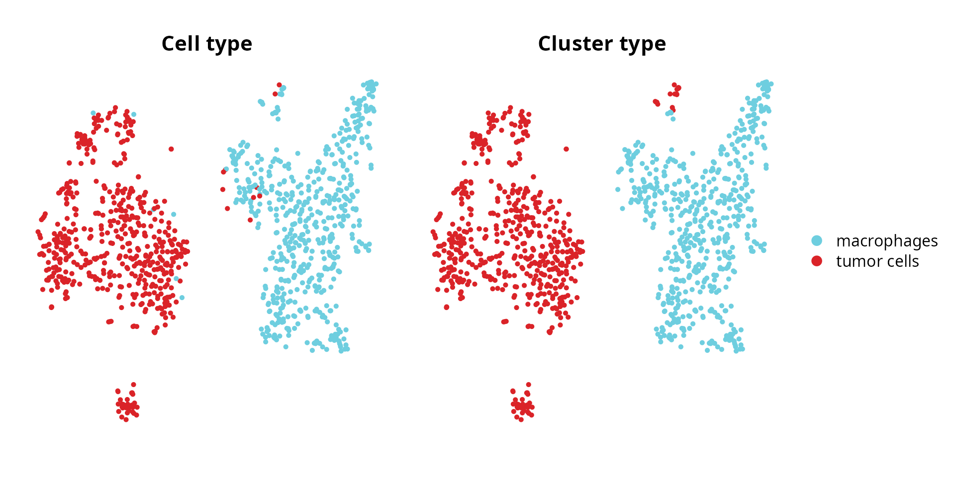
Cell population heterogeneity
We change the cells identity to make the differential expression analysis between clusters.
##
##   0   1   2   3   4   5   6   7
## 379 290 150  85  77  64  33  30
We want to investigate the clusters heterogeneity among macrophages. We identify the clusters annotated as macrophages.
population_oi = "macrophages"

clusters_oi = names(which(cell_type_clusters == population_oi))
clusters_oi
## [1] "0" "3" "5" "7"We represent those clusters on the projection:
aquarius::plot_piechart_subpopulation(
  sobj,
  reduction = name2D,
  big_group_column = "cell_type",
  big_group_of_interest = population_oi,
  big_group_color = color_markers[[population_oi]],
  small_group_column = "seurat_clusters",
  composition_column = "orig.ident",
  composition_color = sample_info$color,
  bg_color = "gray92")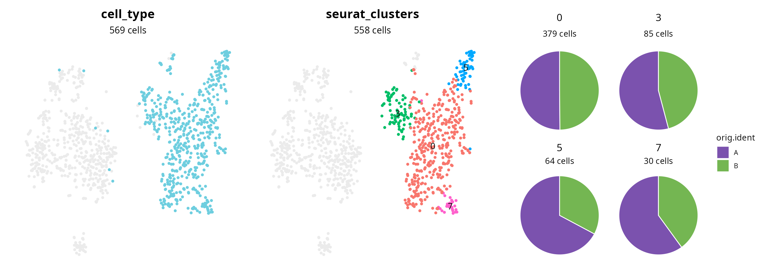
We can see the single-cell level cell type annotation associated with macrophages. Remaining cells are depicted as lightgray cells. In the middle, we see the clusters annotated as macrophages. The piechart shows the representativness of each sample in each cluster. It indicates if comparing clusters together finally corresponds to a comparison between samples. Here, samples are represented within each cluster. So the analysis results may not reflect sample-specific features.
Groups to compare
We set the groups to compare clusters 3 to all others:
group1 = 3
group2 = setdiff(clusters_oi, group1)

aquarius::plot_red_and_blue(sobj, group1, group2, reduction = name2D)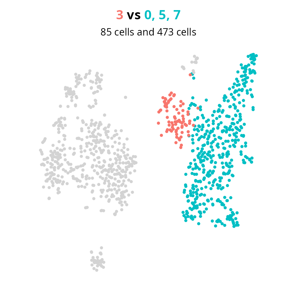
The next step is the differential expression analysis, using, for
instance, Seurat::FindMarkers.
2. Samples
We want to compare the two samples within the macrophages population.
For this, we change the cells identity to consider both the cell type (or cluster type) annotation and the sample of origin.
##
## tumor cells_A macrophages_A macrophages_B tumor cells_B
##           255           308           261           284
We set the groups to compare macrophages in sample A to macrophages in sample B.
group1 = "macrophages_A"
group2 = "macrophages_B"

aquarius::plot_red_and_blue(sobj, group1, group2, reduction = name2D)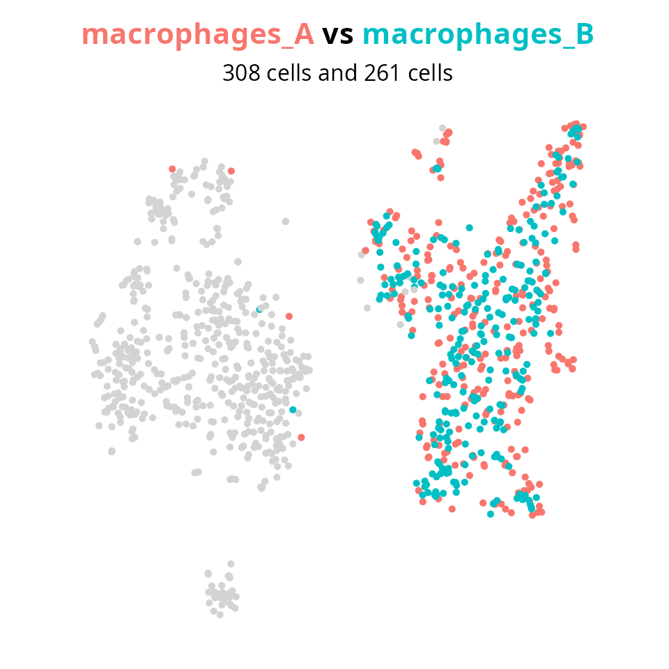
The next step is the differential expression analysis, using, for
instance, Seurat::FindMarkers.
3. Cell types
We want to compare the tumor cells to macrophages.
For this, we change the cells identity the cell type (or cluster type) annotation.
##
## macrophages tumor cells
##         569         539
We set the groups to compare macrophages to other cells.
group1 = "macrophages"
group2 = setdiff(levels(Seurat::Idents(sobj)),
                 group1)

aquarius::plot_red_and_blue(sobj, group1, group2, reduction = name2D)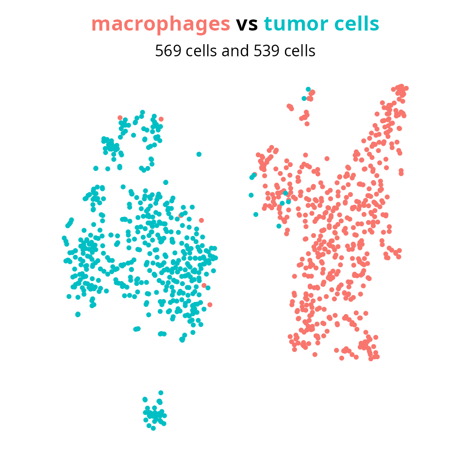
The next step is the differential expression analysis, using, for
instance, Seurat::FindMarkers.
Differential expression analyis
After having defined the two groups of cells to compare, we make the analysis.
Analysis
Here is the chunk we are going to explain
(eval = FALSE):
mark = Seurat::FindMarkers(sobj,
                           ident.1 = group1, ident.2 = group2,
                           min.pct = 0.1)

mark = mark %>%
  dplyr::filter(p_val_adj < 0.05) %>%
  dplyr::arrange(-avg_log2FC, pct.1 - pct.2) %>%
  dplyr::mutate(gene_name = rownames(.))

list_results[[paste0(paste0(group1, collapse = "_"),
                     "_vs_", paste0(group2, collapse = "_"))]] = mark

dim(mark)

head(mark, n = 20)
We identify specific markers for the two groups of interest:
mark = Seurat::FindMarkers(sobj,
                           ident.1 = group1, ident.2 = group2,
                           min.pct = 0.1)

head(mark)
## p_val avg_log2FC pct.1 pct.2 p_val_adj
## Laptm5 4.521799e-184 5.754056 0.960 0.059 6.228327e-180
## Ctss 1.940859e-183 6.176635 0.963 0.089 2.673339e-179
## Fcer1g 1.541759e-182 5.699878 0.960 0.071 2.123619e-178
## Tyrobp 2.425508e-179 6.387295 0.938 0.063 3.340895e-175
## Lyz2 2.807899e-179 6.401865 0.979 0.245 3.867600e-175
## Lcp1 1.530398e-174 5.902032 0.923 0.032 2.107970e-170We filter the table for significantly differentially expressed genes.
Then, we sort the table by fold change and genes specificity The
specificity corresponds to a large difference in the proportion of cells
expressing the features in the group1 compare to the
group2.
mark = mark %>%
  dplyr::filter(p_val_adj < 0.05) %>%
  dplyr::arrange(-avg_log2FC, pct.1 - pct.2) %>%
  dplyr::mutate(gene_name = rownames(.))

dim(mark)
## [1] 3975 6
head(mark)## p_val avg_log2FC pct.1 pct.2 p_val_adj gene_name
## Myo1f 1.432185e-95 9.246354 0.583 0.000 1.972692e-91 Myo1f
## Was 1.116400e-78 8.799830 0.501 0.000 1.537729e-74 Was
## Ly6c2 1.140908e-17 8.736281 0.132 0.002 1.571487e-13 Ly6c2
## Bcl2a1d 7.465725e-43 8.376359 0.299 0.000 1.028329e-38 Bcl2a1d
## Clec12a 3.317522e-129 8.372347 0.735 0.004 4.569555e-125 Clec12a
## Siglece 2.525404e-50 8.326314 0.344 0.000 3.478491e-46 SigleceWe combine the characters string group1 and
group2 to save the results in the list_results
object.
save_name = paste0(paste0(group1, collapse = "_"),
                   "_vs_", paste0(group2, collapse = "_"))
save_name
## [1] "macrophages_vs_tumor cells"
list_results[[save_name]]$de = markVisualization
In this section, we apply diverse functions to visualize the differentially expressed (DE) genes.
Pct plot
We visualize the proportion of cells expressing the DE genes:
aquarius::plot_pct(mark,
                   color_by = "avg_log2FC",
                   label = "gene_name") +
  ggplot2::labs(x = paste0("% of cells expressing in ", group1),
                y = paste0("% of cells expressing in ", group2))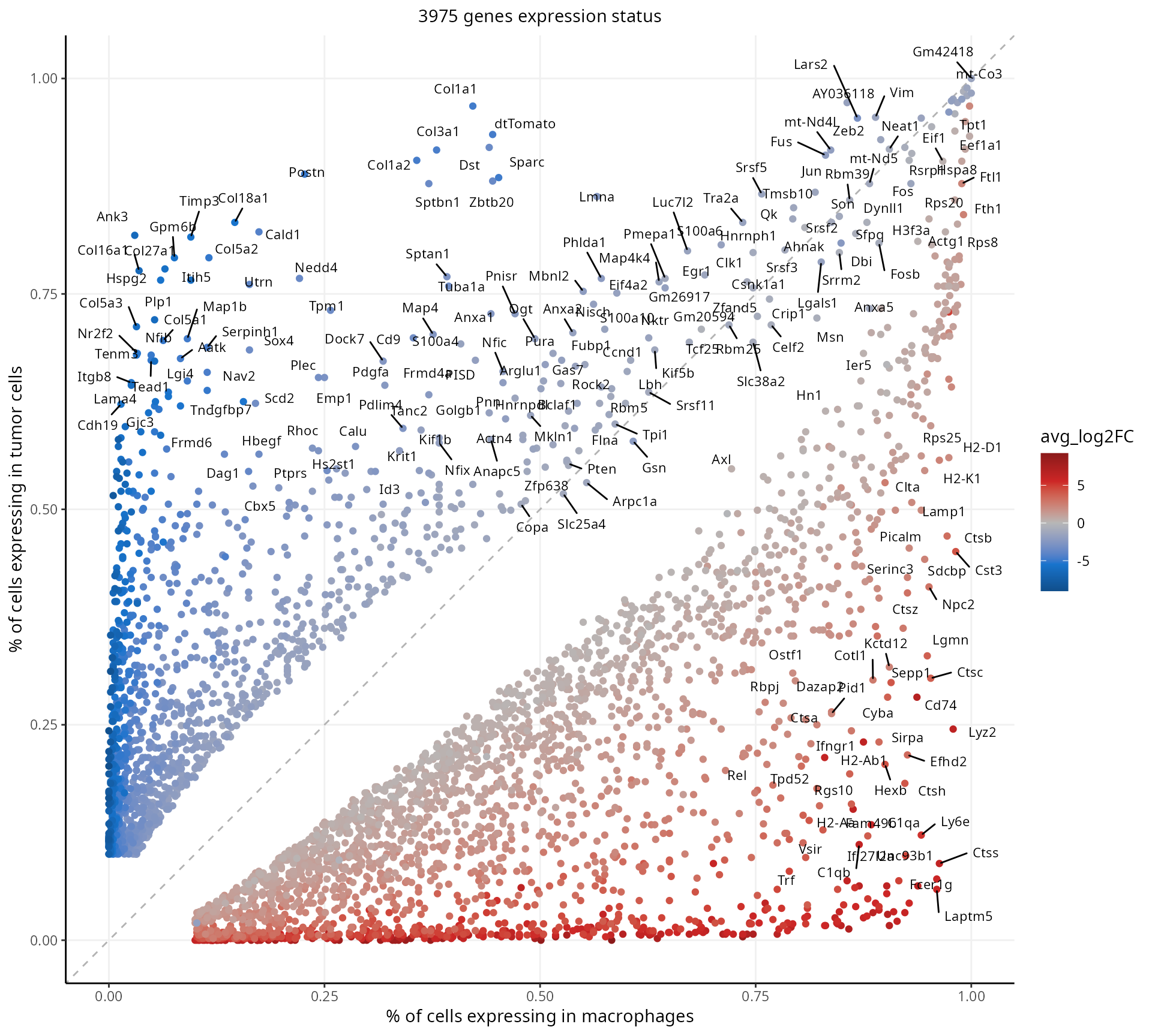
Violin plot
We make violin plots showing the proportion of cells expressing the genes. As example, we choose the Ostf1 gene:
gene_oi = "Ostf1"

mark[gene_oi, ]
## p_val avg_log2FC pct.1 pct.2 p_val_adj gene_name
## Ostf1 7.347424e-70 1.933265 0.793 0.31 1.012034e-65 Ostf1We make a violin plot with default parameters:
aquarius::plot_violin(sobj,
                      feature = gene_oi,
                      group_by = "cell_type")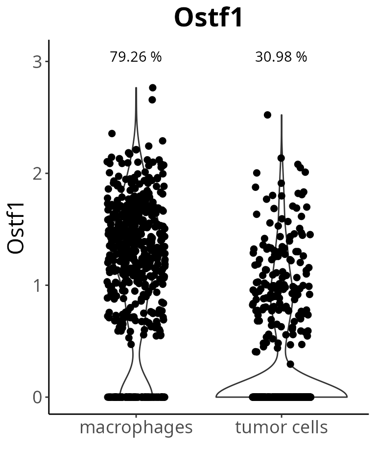
We can color cells by the expression levels of another gene. For instance, one related to proliferation.
aquarius::plot_violin(sobj,
                      feature = gene_oi,
                      group_by = "cell_type",
                      col_by = "Top2a",
                      pt_size = 1)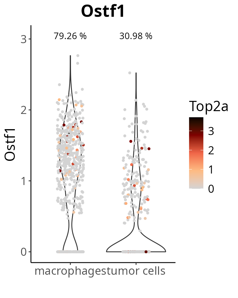
Maybe some cells with 0 expression of Ostf1. We add a noise to visualize this:
aquarius::plot_violin(sobj,
                      feature = gene_oi,
                      group_by = "cell_type",
                      col_by = "Top2a",
                      pt_size = 1,
                      add_noise = TRUE)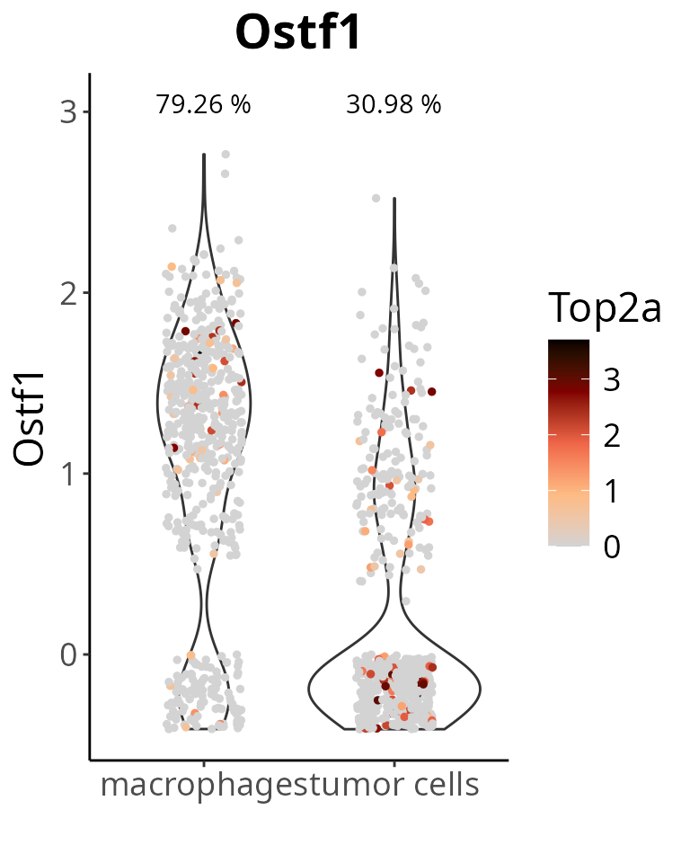
With a whole customized parameter setting, the violin plot could look like:
aquarius::plot_violin(sobj,
                      feature = gene_oi,
                      feature_thresh = 0,
                      group_by = "cell_type",
                      col_by = "Top2a",
                      col_color = RColorBrewer::brewer.pal(name = "Spectral", n = 11),
                      pt_size = 1,
                      text_size = 15,
                      add_noise = TRUE,
                      x_label_angle = 45)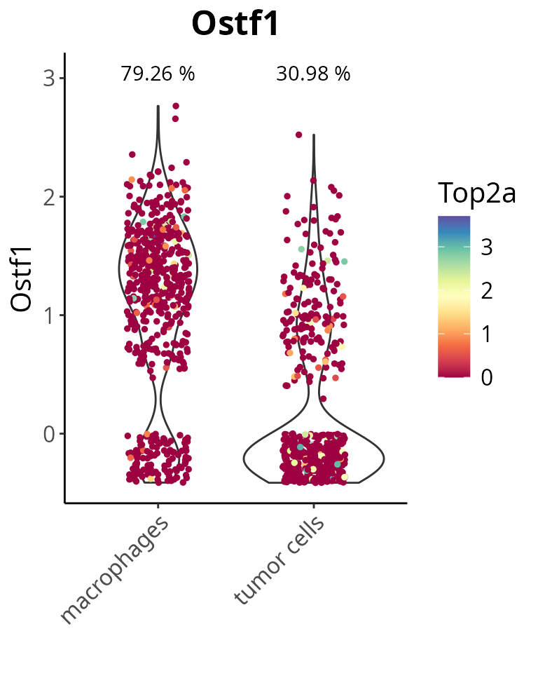
Wordcloud
We visualize the differentially expressed genes as a wordcloud. We
want to size genes by a balance between the fold change and the
proportion of cells expressing the genes. We compute the
FC_x_pct column.
mark = mark %>%
  dplyr::mutate(FC_x_pct = ifelse(avg_log2FC > 0,
                                  yes = avg_log2FC * pct.1,
                                  no = avg_log2FC * pct.2)) %>%
  dplyr::filter(FC_x_pct != 0)

head(mark)
## p_val avg_log2FC pct.1 pct.2 p_val_adj gene_name FC_x_pct
## Myo1f 1.432185e-95 9.246354 0.583 0.000 1.972692e-91 Myo1f 5.390625
## Was 1.116400e-78 8.799830 0.501 0.000 1.537729e-74 Was 4.408715
## Ly6c2 1.140908e-17 8.736281 0.132 0.002 1.571487e-13 Ly6c2 1.153189
## Bcl2a1d 7.465725e-43 8.376359 0.299 0.000 1.028329e-38 Bcl2a1d 2.504531
## Clec12a 3.317522e-129 8.372347 0.735 0.004 4.569555e-125 Clec12a 6.153675
## Siglece 2.525404e-50 8.326314 0.344 0.000 3.478491e-46 Siglece 2.864252We make two wordclouds, for the up-regulated (left) and down-regulated (right) genes.
# Up-regulated in group1 compared to group2
p1 = mark %>%
  dplyr::filter(avg_log2FC > 0) %>%
  dplyr::top_n(., n = 200, wt = FC_x_pct) %>%
  aquarius::plot_wordcloud(.,
                           label = "gene_name",
                           size_by = "avg_log2FC",
                           max_size = 9,
                           color_by = "FC_x_pct") +
  ggplot2::labs(title = paste0(sum(mark$avg_log2FC > 0), " up-regulated genes"),
                subtitle = paste0("in ", paste0(group1, collapse = ", "),
                                  " compared to ", paste0(group2, collapse = ", "))) +
  ggplot2::theme(plot.title = element_text(face = "bold"),
                 plot.subtitle = element_text(hjust = 0.5))

# Up-regulated in group2 compared to group1
p2 = mark %>%
  dplyr::filter(avg_log2FC < 0) %>%
  dplyr::top_n(., n = 200, wt = -FC_x_pct) %>%
  aquarius::plot_wordcloud(.,
                           label = "gene_name",
                           size_by = "avg_log2FC",
                           max_size = 5,
                           color_by = "FC_x_pct") +
  ggplot2::labs(title = paste0(sum(mark$avg_log2FC < 0), " up-regulated genes"),
                subtitle = paste0("in ", paste0(group2, collapse = ", "),
                                  " compared to ", paste0(group1, collapse = ", "))) +
  ggplot2::theme(plot.title = element_text(face = "bold"),
                 plot.subtitle = element_text(hjust = 0.5))

# Assemble
p1 | p2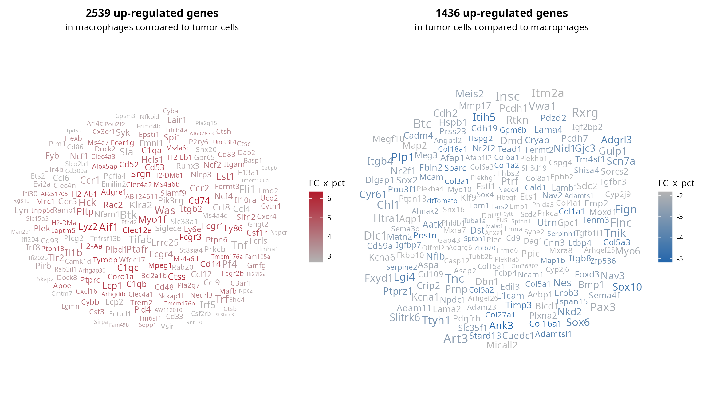
Over Representation Analysis
As an example, we consider ORA for the up-regulated genes only:
## [1] "Myo1f" "Was" "Ly6c2" "Bcl2a1d" "Clec12a" "Siglece"Analysis
We make the over-representation analysis. The function automatically convert gene names to gene identifiers to interact with a database.
enrichr_results = aquarius::run_enrichr(gene_names = gene_oi,
                                        gene_corresp = gene_corresp,
                                        gene_sets = gene_sets[, c("gs_name", "ensembl_gene")],
                                        make_plot = TRUE,
                                        plot_title = paste0("Up-regulated in ", group1,
                                                            " compared to ", group2))

names(enrichr_results)
## [1] "ego" "plot"
list_results[[save_name]]$up$enrichr = enrichr_results$egoVisualization
With clusterProfiler
A plot is stored in the results:
enrichr_results$plot +
  ggplot2::theme(axis.text.y = element_text(size = 8))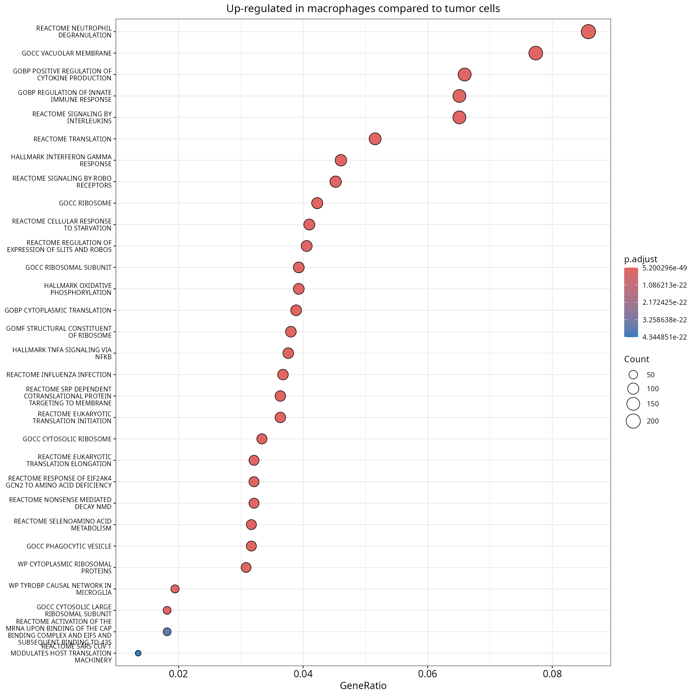
Wordcloud
The enrichr result is a dataframe looking like:
head(enrichr_results$ego@result)## ID
## REACTOME_SRP_DEPENDENT_COTRANSLATIONAL_PROTEIN_TARGETING_TO_MEMBRANE REACTOME_SRP_DEPENDENT_COTRANSLATIONAL_PROTEIN_TARGETING_TO_MEMBRANE
## REACTOME_NEUTROPHIL_DEGRANULATION REACTOME_NEUTROPHIL_DEGRANULATION
## REACTOME_EUKARYOTIC_TRANSLATION_ELONGATION REACTOME_EUKARYOTIC_TRANSLATION_ELONGATION
## WP_CYTOPLASMIC_RIBOSOMAL_PROTEINS WP_CYTOPLASMIC_RIBOSOMAL_PROTEINS
## REACTOME_EUKARYOTIC_TRANSLATION_INITIATION REACTOME_EUKARYOTIC_TRANSLATION_INITIATION
## REACTOME_RESPONSE_OF_EIF2AK4_GCN2_TO_AMINO_ACID_DEFICIENCY REACTOME_RESPONSE_OF_EIF2AK4_GCN2_TO_AMINO_ACID_DEFICIENCY
## Description
## REACTOME_SRP_DEPENDENT_COTRANSLATIONAL_PROTEIN_TARGETING_TO_MEMBRANE REACTOME_SRP_DEPENDENT_COTRANSLATIONAL_PROTEIN_TARGETING_TO_MEMBRANE
## REACTOME_NEUTROPHIL_DEGRANULATION REACTOME_NEUTROPHIL_DEGRANULATION
## REACTOME_EUKARYOTIC_TRANSLATION_ELONGATION REACTOME_EUKARYOTIC_TRANSLATION_ELONGATION
## WP_CYTOPLASMIC_RIBOSOMAL_PROTEINS WP_CYTOPLASMIC_RIBOSOMAL_PROTEINS
## REACTOME_EUKARYOTIC_TRANSLATION_INITIATION REACTOME_EUKARYOTIC_TRANSLATION_INITIATION
## REACTOME_RESPONSE_OF_EIF2AK4_GCN2_TO_AMINO_ACID_DEFICIENCY REACTOME_RESPONSE_OF_EIF2AK4_GCN2_TO_AMINO_ACID_DEFICIENCY
## GeneRatio
## REACTOME_SRP_DEPENDENT_COTRANSLATIONAL_PROTEIN_TARGETING_TO_MEMBRANE 86/2366
## REACTOME_NEUTROPHIL_DEGRANULATION 203/2366
## REACTOME_EUKARYOTIC_TRANSLATION_ELONGATION 76/2366
## WP_CYTOPLASMIC_RIBOSOMAL_PROTEINS 73/2366
## REACTOME_EUKARYOTIC_TRANSLATION_INITIATION 86/2366
## REACTOME_RESPONSE_OF_EIF2AK4_GCN2_TO_AMINO_ACID_DEFICIENCY 76/2366
## BgRatio
## REACTOME_SRP_DEPENDENT_COTRANSLATIONAL_PROTEIN_TARGETING_TO_MEMBRANE 109/16961
## REACTOME_NEUTROPHIL_DEGRANULATION 492/16961
## REACTOME_EUKARYOTIC_TRANSLATION_ELONGATION 90/16961
## WP_CYTOPLASMIC_RIBOSOMAL_PROTEINS 86/16961
## REACTOME_EUKARYOTIC_TRANSLATION_INITIATION 117/16961
## REACTOME_RESPONSE_OF_EIF2AK4_GCN2_TO_AMINO_ACID_DEFICIENCY 98/16961
## RichFactor
## REACTOME_SRP_DEPENDENT_COTRANSLATIONAL_PROTEIN_TARGETING_TO_MEMBRANE 0.7889908
## REACTOME_NEUTROPHIL_DEGRANULATION 0.4126016
## REACTOME_EUKARYOTIC_TRANSLATION_ELONGATION 0.8444444
## WP_CYTOPLASMIC_RIBOSOMAL_PROTEINS 0.8488372
## REACTOME_EUKARYOTIC_TRANSLATION_INITIATION 0.7350427
## REACTOME_RESPONSE_OF_EIF2AK4_GCN2_TO_AMINO_ACID_DEFICIENCY 0.7755102
## FoldEnrichment
## REACTOME_SRP_DEPENDENT_COTRANSLATIONAL_PROTEIN_TARGETING_TO_MEMBRANE 5.655990
## REACTOME_NEUTROPHIL_DEGRANULATION 2.957792
## REACTOME_EUKARYOTIC_TRANSLATION_ELONGATION 6.053517
## WP_CYTOPLASMIC_RIBOSOMAL_PROTEINS 6.085008
## REACTOME_EUKARYOTIC_TRANSLATION_INITIATION 5.269256
## REACTOME_RESPONSE_OF_EIF2AK4_GCN2_TO_AMINO_ACID_DEFICIENCY 5.559353
## zScore
## REACTOME_SRP_DEPENDENT_COTRANSLATIONAL_PROTEIN_TARGETING_TO_MEMBRANE 19.63441
## REACTOME_NEUTROPHIL_DEGRANULATION 17.74327
## REACTOME_EUKARYOTIC_TRANSLATION_ELONGATION 19.35365
## WP_CYTOPLASMIC_RIBOSOMAL_PROTEINS 19.03431
## REACTOME_EUKARYOTIC_TRANSLATION_INITIATION 18.65695
## REACTOME_RESPONSE_OF_EIF2AK4_GCN2_TO_AMINO_ACID_DEFICIENCY 18.22498
## pvalue
## REACTOME_SRP_DEPENDENT_COTRANSLATIONAL_PROTEIN_TARGETING_TO_MEMBRANE 5.986297e-53
## REACTOME_NEUTROPHIL_DEGRANULATION 9.621070e-52
## REACTOME_EUKARYOTIC_TRANSLATION_ELONGATION 4.104214e-51
## WP_CYTOPLASMIC_RIBOSOMAL_PROTEINS 1.822948e-49
## REACTOME_EUKARYOTIC_TRANSLATION_INITIATION 1.641639e-48
## REACTOME_RESPONSE_OF_EIF2AK4_GCN2_TO_AMINO_ACID_DEFICIENCY 6.393024e-46
## p.adjust
## REACTOME_SRP_DEPENDENT_COTRANSLATIONAL_PROTEIN_TARGETING_TO_MEMBRANE 5.200296e-49
## REACTOME_NEUTROPHIL_DEGRANULATION 4.178912e-48
## REACTOME_EUKARYOTIC_TRANSLATION_ELONGATION 1.188444e-47
## WP_CYTOPLASMIC_RIBOSOMAL_PROTEINS 3.958987e-46
## REACTOME_EUKARYOTIC_TRANSLATION_INITIATION 2.852183e-45
## REACTOME_RESPONSE_OF_EIF2AK4_GCN2_TO_AMINO_ACID_DEFICIENCY 9.256033e-43
## qvalue
## REACTOME_SRP_DEPENDENT_COTRANSLATIONAL_PROTEIN_TARGETING_TO_MEMBRANE 3.697011e-49
## REACTOME_NEUTROPHIL_DEGRANULATION 2.970885e-48
## REACTOME_EUKARYOTIC_TRANSLATION_ELONGATION 8.448920e-48
## WP_CYTOPLASMIC_RIBOSOMAL_PROTEINS 2.814536e-46
## REACTOME_EUKARYOTIC_TRANSLATION_INITIATION 2.027683e-45
## REACTOME_RESPONSE_OF_EIF2AK4_GCN2_TO_AMINO_ACID_DEFICIENCY 6.580328e-43
## geneID
## REACTOME_SRP_DEPENDENT_COTRANSLATIONAL_PROTEIN_TARGETING_TO_MEMBRANE ENSMUSG00000025935/ENSMUSG00000043716/ENSMUSG00000073702/ENSMUSG00000046330/ENSMUSG00000026511/ENSMUSG00000062647/ENSMUSG00000038900/ENSMUSG00000062997/ENSMUSG00000009549/ENSMUSG00000027642/ENSMUSG00000039001/ENSMUSG00000079641/ENSMUSG00000002014/ENSMUSG00000031320/ENSMUSG00000079435/ENSMUSG00000028081/ENSMUSG00000090733/ENSMUSG00000062006/ENSMUSG00000028234/ENSMUSG00000053317/ENSMUSG00000028495/ENSMUSG00000047675/ENSMUSG00000059291/ENSMUSG00000028757/ENSMUSG00000028936/ENSMUSG00000047215/ENSMUSG00000058558/ENSMUSG00000067274/ENSMUSG00000041453/ENSMUSG00000030062/ENSMUSG00000057841/ENSMUSG00000006333/ENSMUSG00000030432/ENSMUSG00000012848/ENSMUSG00000040952/ENSMUSG00000037563/ENSMUSG00000003429/ENSMUSG00000074129/ENSMUSG00000059070/ENSMUSG00000061787/ENSMUSG00000030744/ENSMUSG00000035227/ENSMUSG00000046364/ENSMUSG00000090862/ENSMUSG00000008683/ENSMUSG00000025508/ENSMUSG00000063457/ENSMUSG00000025362/ENSMUSG00000054408/ENSMUSG00000045128/ENSMUSG00000000740/ENSMUSG00000012405/ENSMUSG00000025290/ENSMUSG00000021917/ENSMUSG00000009927/ENSMUSG00000007892/ENSMUSG00000032399/ENSMUSG00000048758/ENSMUSG00000032518/ENSMUSG00000025794/ENSMUSG00000078974/ENSMUSG00000020460/ENSMUSG00000060938/ENSMUSG00000071415/ENSMUSG00000017404/ENSMUSG00000057322/ENSMUSG00000049517/ENSMUSG00000061477/ENSMUSG00000034892/ENSMUSG00000049751/ENSMUSG00000041841/ENSMUSG00000058600/ENSMUSG00000003970/ENSMUSG00000060036/ENSMUSG00000060636/ENSMUSG00000098274/ENSMUSG00000044533/ENSMUSG00000052146/ENSMUSG00000037805/ENSMUSG00000067288/ENSMUSG00000008668/ENSMUSG00000057863/ENSMUSG00000024608/ENSMUSG00000024516/ENSMUSG00000062328/ENSMUSG00000038274
## REACTOME_NEUTROPHIL_DEGRANULATION ENSMUSG00000025950/ENSMUSG00000026177/ENSMUSG00000036707/ENSMUSG00000026395/ENSMUSG00000008475/ENSMUSG00000040713/ENSMUSG00000026656/ENSMUSG00000059089/ENSMUSG00000058715/ENSMUSG00000003458/ENSMUSG00000073489/ENSMUSG00000090272/ENSMUSG00000038633/ENSMUSG00000026958/ENSMUSG00000014867/ENSMUSG00000026878/ENSMUSG00000026880/ENSMUSG00000026914/ENSMUSG00000025314/ENSMUSG00000027187/ENSMUSG00000009549/ENSMUSG00000027287/ENSMUSG00000060802/ENSMUSG00000060131/ENSMUSG00000037902/ENSMUSG00000027435/ENSMUSG00000027447/ENSMUSG00000033059/ENSMUSG00000017760/ENSMUSG00000016256/ENSMUSG00000000826/ENSMUSG00000015340/ENSMUSG00000031007/ENSMUSG00000000787/ENSMUSG00000001128/ENSMUSG00000016534/ENSMUSG00000050029/ENSMUSG00000019088/ENSMUSG00000031266/ENSMUSG00000061778/ENSMUSG00000095788/ENSMUSG00000019528/ENSMUSG00000042997/ENSMUSG00000027995/ENSMUSG00000028062/ENSMUSG00000038642/ENSMUSG00000068798/ENSMUSG00000040747/ENSMUSG00000068749/ENSMUSG00000028164/ENSMUSG00000028163/ENSMUSG00000091512/ENSMUSG00000028249/ENSMUSG00000028228/ENSMUSG00000073987/ENSMUSG00000028413/ENSMUSG00000028656/ENSMUSG00000056529/ENSMUSG00000028874/ENSMUSG00000028673/ENSMUSG00000028757/ENSMUSG00000028599/ENSMUSG00000028931/ENSMUSG00000039899/ENSMUSG00000029082/ENSMUSG00000029171/ENSMUSG00000058427/ENSMUSG00000029322/ENSMUSG00000035273/ENSMUSG00000064267/ENSMUSG00000029416/ENSMUSG00000025534/ENSMUSG00000001847/ENSMUSG00000047843/ENSMUSG00000029915/ENSMUSG00000050732/ENSMUSG00000079477/ENSMUSG00000025701/ENSMUSG00000040552/ENSMUSG00000030147/ENSMUSG00000030144/ENSMUSG00000004266/ENSMUSG00000053063/ENSMUSG00000030225/ENSMUSG00000008540/ENSMUSG00000030263/ENSMUSG00000058818/ENSMUSG00000055541/ENSMUSG00000049130/ENSMUSG00000046223/ENSMUSG00000060791/ENSMUSG00000030579/ENSMUSG00000036427/ENSMUSG00000004609/ENSMUSG00000030474/ENSMUSG00000050708/ENSMUSG00000030447/ENSMUSG00000030560/ENSMUSG00000061119/ENSMUSG00000030647/ENSMUSG00000032725/ENSMUSG00000030842/ENSMUSG00000073982/ENSMUSG00000030830/ENSMUSG00000030793/ENSMUSG00000030786/ENSMUSG00000030789/ENSMUSG00000025473/ENSMUSG00000002957/ENSMUSG00000007891/ENSMUSG00000019810/ENSMUSG00000004207/ENSMUSG00000000290/ENSMUSG00000009292/ENSMUSG00000020277/ENSMUSG00000005054/ENSMUSG00000032788/ENSMUSG00000035697/ENSMUSG00000069516/ENSMUSG00000052681/ENSMUSG00000034707/ENSMUSG00000040345/ENSMUSG00000013974/ENSMUSG00000031447/ENSMUSG00000037260/ENSMUSG00000031591/ENSMUSG00000046718/ENSMUSG00000002885/ENSMUSG00000005142/ENSMUSG00000031722/ENSMUSG00000031729/ENSMUSG00000031827/ENSMUSG00000006519/ENSMUSG00000006589/ENSMUSG00000021822/ENSMUSG00000021948/ENSMUSG00000037824/ENSMUSG00000021939/ENSMUSG00000022136/ENSMUSG00000015656/ENSMUSG00000032294/ENSMUSG00000050721/ENSMUSG00000054693/ENSMUSG00000037742/ENSMUSG00000032359/ENSMUSG00000032560/ENSMUSG00000045594/ENSMUSG00000032435/ENSMUSG00000032434/ENSMUSG00000020476/ENSMUSG00000020152/ENSMUSG00000020272/ENSMUSG00000020143/ENSMUSG00000000594/ENSMUSG00000049299/ENSMUSG00000018774/ENSMUSG00000020917/ENSMUSG00000019173/ENSMUSG00000019302/ENSMUSG00000034708/ENSMUSG00000034652/ENSMUSG00000025575/ENSMUSG00000025579/ENSMUSG00000021218/ENSMUSG00000015671/ENSMUSG00000025877/ENSMUSG00000035711/ENSMUSG00000042082/ENSMUSG00000021687/ENSMUSG00000021665/ENSMUSG00000021069/ENSMUSG00000021114/ENSMUSG00000021242/ENSMUSG00000022575/ENSMUSG00000022415/ENSMUSG00000058099/ENSMUSG00000022620/ENSMUSG00000098112/ENSMUSG00000022488/ENSMUSG00000004070/ENSMUSG00000022765/ENSMUSG00000055447/ENSMUSG00000025613/ENSMUSG00000095687/ENSMUSG00000014769/ENSMUSG00000053436/ENSMUSG00000007038/ENSMUSG00000024387/ENSMUSG00000073411/ENSMUSG00000060550/ENSMUSG00000024164/ENSMUSG00000024091/ENSMUSG00000056515/ENSMUSG00000039770/ENSMUSG00000024349/ENSMUSG00000051439/ENSMUSG00000024456/ENSMUSG00000056130/ENSMUSG00000001750/ENSMUSG00000024885/ENSMUSG00000024661/ENSMUSG00000024725/ENSMUSG00000011752
## REACTOME_EUKARYOTIC_TRANSLATION_ELONGATION ENSMUSG00000043716/ENSMUSG00000073702/ENSMUSG00000025967/ENSMUSG00000046330/ENSMUSG00000062647/ENSMUSG00000038900/ENSMUSG00000062997/ENSMUSG00000039001/ENSMUSG00000079641/ENSMUSG00000031320/ENSMUSG00000079435/ENSMUSG00000028081/ENSMUSG00000090733/ENSMUSG00000062006/ENSMUSG00000028234/ENSMUSG00000028495/ENSMUSG00000047675/ENSMUSG00000059291/ENSMUSG00000028936/ENSMUSG00000047215/ENSMUSG00000058558/ENSMUSG00000067274/ENSMUSG00000041453/ENSMUSG00000057841/ENSMUSG00000006333/ENSMUSG00000030432/ENSMUSG00000012848/ENSMUSG00000040952/ENSMUSG00000037563/ENSMUSG00000003429/ENSMUSG00000074129/ENSMUSG00000059070/ENSMUSG00000061787/ENSMUSG00000030744/ENSMUSG00000046364/ENSMUSG00000090862/ENSMUSG00000008683/ENSMUSG00000025508/ENSMUSG00000063457/ENSMUSG00000025362/ENSMUSG00000045128/ENSMUSG00000000740/ENSMUSG00000012405/ENSMUSG00000025290/ENSMUSG00000009927/ENSMUSG00000007892/ENSMUSG00000032399/ENSMUSG00000037742/ENSMUSG00000048758/ENSMUSG00000032518/ENSMUSG00000025794/ENSMUSG00000020460/ENSMUSG00000060938/ENSMUSG00000071415/ENSMUSG00000017404/ENSMUSG00000057322/ENSMUSG00000049517/ENSMUSG00000061477/ENSMUSG00000034892/ENSMUSG00000049751/ENSMUSG00000041841/ENSMUSG00000058600/ENSMUSG00000003970/ENSMUSG00000060036/ENSMUSG00000060636/ENSMUSG00000098274/ENSMUSG00000044533/ENSMUSG00000052146/ENSMUSG00000037805/ENSMUSG00000067288/ENSMUSG00000008668/ENSMUSG00000057863/ENSMUSG00000024608/ENSMUSG00000062328/ENSMUSG00000038274/ENSMUSG00000071644
## WP_CYTOPLASMIC_RIBOSOMAL_PROTEINS ENSMUSG00000043716/ENSMUSG00000073702/ENSMUSG00000046330/ENSMUSG00000062647/ENSMUSG00000038900/ENSMUSG00000062997/ENSMUSG00000039001/ENSMUSG00000079641/ENSMUSG00000031320/ENSMUSG00000079435/ENSMUSG00000028081/ENSMUSG00000090733/ENSMUSG00000062006/ENSMUSG00000028234/ENSMUSG00000028495/ENSMUSG00000047675/ENSMUSG00000003644/ENSMUSG00000059291/ENSMUSG00000028936/ENSMUSG00000047215/ENSMUSG00000058558/ENSMUSG00000067274/ENSMUSG00000041453/ENSMUSG00000057841/ENSMUSG00000006333/ENSMUSG00000030432/ENSMUSG00000012848/ENSMUSG00000040952/ENSMUSG00000037563/ENSMUSG00000003429/ENSMUSG00000074129/ENSMUSG00000059070/ENSMUSG00000061787/ENSMUSG00000030744/ENSMUSG00000046364/ENSMUSG00000090862/ENSMUSG00000008683/ENSMUSG00000025508/ENSMUSG00000063457/ENSMUSG00000025362/ENSMUSG00000045128/ENSMUSG00000000740/ENSMUSG00000012405/ENSMUSG00000025290/ENSMUSG00000009927/ENSMUSG00000007892/ENSMUSG00000032399/ENSMUSG00000048758/ENSMUSG00000032518/ENSMUSG00000025794/ENSMUSG00000020460/ENSMUSG00000060938/ENSMUSG00000071415/ENSMUSG00000017404/ENSMUSG00000057322/ENSMUSG00000049517/ENSMUSG00000061477/ENSMUSG00000034892/ENSMUSG00000041841/ENSMUSG00000058600/ENSMUSG00000003970/ENSMUSG00000060036/ENSMUSG00000060636/ENSMUSG00000098274/ENSMUSG00000044533/ENSMUSG00000052146/ENSMUSG00000037805/ENSMUSG00000067288/ENSMUSG00000008668/ENSMUSG00000057863/ENSMUSG00000024608/ENSMUSG00000062328/ENSMUSG00000038274
## REACTOME_EUKARYOTIC_TRANSLATION_INITIATION ENSMUSG00000043716/ENSMUSG00000073702/ENSMUSG00000046330/ENSMUSG00000062647/ENSMUSG00000038900/ENSMUSG00000062997/ENSMUSG00000027170/ENSMUSG00000039001/ENSMUSG00000079641/ENSMUSG00000031320/ENSMUSG00000079435/ENSMUSG00000028081/ENSMUSG00000090733/ENSMUSG00000062006/ENSMUSG00000028156/ENSMUSG00000028234/ENSMUSG00000028495/ENSMUSG00000047675/ENSMUSG00000028798/ENSMUSG00000059291/ENSMUSG00000028936/ENSMUSG00000047215/ENSMUSG00000058558/ENSMUSG00000067274/ENSMUSG00000041453/ENSMUSG00000057841/ENSMUSG00000006333/ENSMUSG00000030432/ENSMUSG00000012848/ENSMUSG00000040952/ENSMUSG00000037563/ENSMUSG00000053565/ENSMUSG00000003429/ENSMUSG00000074129/ENSMUSG00000059070/ENSMUSG00000061787/ENSMUSG00000030744/ENSMUSG00000031029/ENSMUSG00000046364/ENSMUSG00000090862/ENSMUSG00000008683/ENSMUSG00000030738/ENSMUSG00000025508/ENSMUSG00000063457/ENSMUSG00000025362/ENSMUSG00000031490/ENSMUSG00000045128/ENSMUSG00000000740/ENSMUSG00000012405/ENSMUSG00000025290/ENSMUSG00000009927/ENSMUSG00000007892/ENSMUSG00000032399/ENSMUSG00000048758/ENSMUSG00000032518/ENSMUSG00000025794/ENSMUSG00000020460/ENSMUSG00000060938/ENSMUSG00000071415/ENSMUSG00000017404/ENSMUSG00000057322/ENSMUSG00000049517/ENSMUSG00000061477/ENSMUSG00000034892/ENSMUSG00000049751/ENSMUSG00000021282/ENSMUSG00000041841/ENSMUSG00000058600/ENSMUSG00000022336/ENSMUSG00000022312/ENSMUSG00000003970/ENSMUSG00000016554/ENSMUSG00000033047/ENSMUSG00000060036/ENSMUSG00000058655/ENSMUSG00000060636/ENSMUSG00000098274/ENSMUSG00000044533/ENSMUSG00000052146/ENSMUSG00000037805/ENSMUSG00000067288/ENSMUSG00000008668/ENSMUSG00000057863/ENSMUSG00000024608/ENSMUSG00000062328/ENSMUSG00000038274
## REACTOME_RESPONSE_OF_EIF2AK4_GCN2_TO_AMINO_ACID_DEFICIENCY ENSMUSG00000043716/ENSMUSG00000073702/ENSMUSG00000046330/ENSMUSG00000026628/ENSMUSG00000062647/ENSMUSG00000038900/ENSMUSG00000062997/ENSMUSG00000056501/ENSMUSG00000039001/ENSMUSG00000079641/ENSMUSG00000031320/ENSMUSG00000079435/ENSMUSG00000028081/ENSMUSG00000090733/ENSMUSG00000062006/ENSMUSG00000028234/ENSMUSG00000028495/ENSMUSG00000047675/ENSMUSG00000059291/ENSMUSG00000028936/ENSMUSG00000047215/ENSMUSG00000058558/ENSMUSG00000067274/ENSMUSG00000041453/ENSMUSG00000057841/ENSMUSG00000006333/ENSMUSG00000030432/ENSMUSG00000012848/ENSMUSG00000040952/ENSMUSG00000037563/ENSMUSG00000003429/ENSMUSG00000074129/ENSMUSG00000059070/ENSMUSG00000061787/ENSMUSG00000030744/ENSMUSG00000046364/ENSMUSG00000090862/ENSMUSG00000008683/ENSMUSG00000025508/ENSMUSG00000063457/ENSMUSG00000025362/ENSMUSG00000045128/ENSMUSG00000000740/ENSMUSG00000012405/ENSMUSG00000025290/ENSMUSG00000009927/ENSMUSG00000007892/ENSMUSG00000032399/ENSMUSG00000048758/ENSMUSG00000032518/ENSMUSG00000025794/ENSMUSG00000020460/ENSMUSG00000060938/ENSMUSG00000071415/ENSMUSG00000017404/ENSMUSG00000057322/ENSMUSG00000049517/ENSMUSG00000061477/ENSMUSG00000034892/ENSMUSG00000049751/ENSMUSG00000041841/ENSMUSG00000058600/ENSMUSG00000003970/ENSMUSG00000060036/ENSMUSG00000060636/ENSMUSG00000098274/ENSMUSG00000044533/ENSMUSG00000052146/ENSMUSG00000037805/ENSMUSG00000067288/ENSMUSG00000008668/ENSMUSG00000057863/ENSMUSG00000024423/ENSMUSG00000024608/ENSMUSG00000062328/ENSMUSG00000038274
## Count
## REACTOME_SRP_DEPENDENT_COTRANSLATIONAL_PROTEIN_TARGETING_TO_MEMBRANE 86
## REACTOME_NEUTROPHIL_DEGRANULATION 203
## REACTOME_EUKARYOTIC_TRANSLATION_ELONGATION 76
## WP_CYTOPLASMIC_RIBOSOMAL_PROTEINS 73
## REACTOME_EUKARYOTIC_TRANSLATION_INITIATION 86
## REACTOME_RESPONSE_OF_EIF2AK4_GCN2_TO_AMINO_ACID_DEFICIENCY 76We want to make a word cloud to identify the redundant gene sets. First, we select gene sets of interest:
gene_sets_oi = enrichr_results$ego@result %>%
  dplyr::filter(p.adjust < 0.01) %>%
  dplyr::pull(ID)

head(gene_sets_oi)
## [1] "REACTOME_SRP_DEPENDENT_COTRANSLATIONAL_PROTEIN_TARGETING_TO_MEMBRANE"
## [2] "REACTOME_NEUTROPHIL_DEGRANULATION"
## [3] "REACTOME_EUKARYOTIC_TRANSLATION_ELONGATION"
## [4] "WP_CYTOPLASMIC_RIBOSOMAL_PROTEINS"
## [5] "REACTOME_EUKARYOTIC_TRANSLATION_INITIATION"
## [6] "REACTOME_RESPONSE_OF_EIF2AK4_GCN2_TO_AMINO_ACID_DEFICIENCY"
length(gene_sets_oi)## [1] 1422We extract and content the words:
not_of_interest = c("OF", "AND", "IN", "BY", "TO", "THE",
                    "POSITIVE", "NEGATIVE", "REGULATION", "ACTIVITY", "CELL",
                    "PROCESS", "SIGNALING", "RESPONSE", "PATHWAY", "PROTEIN")

gs_to_plot = lapply(gene_sets_oi, FUN = function(gs_name) {
  gs_name_cut = stringr::str_split(gs_name, pattern = "_") %>%
    # Remove the first word (REACTOME, GOBP...)
    lapply(., FUN = function(x) x[-1]) %>%
    unlist()

  # Remove non-interesting words
  gs_name_cut = gs_name_cut[!(gs_name_cut %in% not_of_interest)]

  # Remove number
  is_number = grep(gs_name_cut,
                   pattern = "^[0-9][0-9]*$",
                   value = TRUE)
  gs_name_cut = gs_name_cut[!(gs_name_cut %in% is_number)]

  return(gs_name_cut)

}) %>% # Make a dataframe counting the words
  unlist() %>%
  table() %>%
  as.data.frame.table() %>%
  `colnames<-`(c("Word", "Count")) %>%
  # Remove low count
  dplyr::filter(Count > 1)

head(gs_to_plot)
## Word Count
## 1 2PATHWAY 2
## 2 A 5
## 3 ABC 2
## 4 ACID 10
## 5 ACIDIFICATION 5
## 6 ACIDS 4
nrow(gs_to_plot)## [1] 531We make a wordcloud:
aquarius::plot_wordcloud(gs_to_plot,
                         label = "Word",
                         size_by = "Count",
                         size_limit = 0.9,
                         max_size = 9,
                         color_by = "Count",
                         color_palette = aquarius::palette_GrOrBl) +
  ggplot2::labs(title = paste0("Gene sets enriched in ", group1),
                subtitle = paste0(length(gene_sets_oi), " gene sets")) +
  ggplot2::theme(plot.title = element_text(face = "bold"),
                 plot.subtitle = element_text(hjust = 0.5))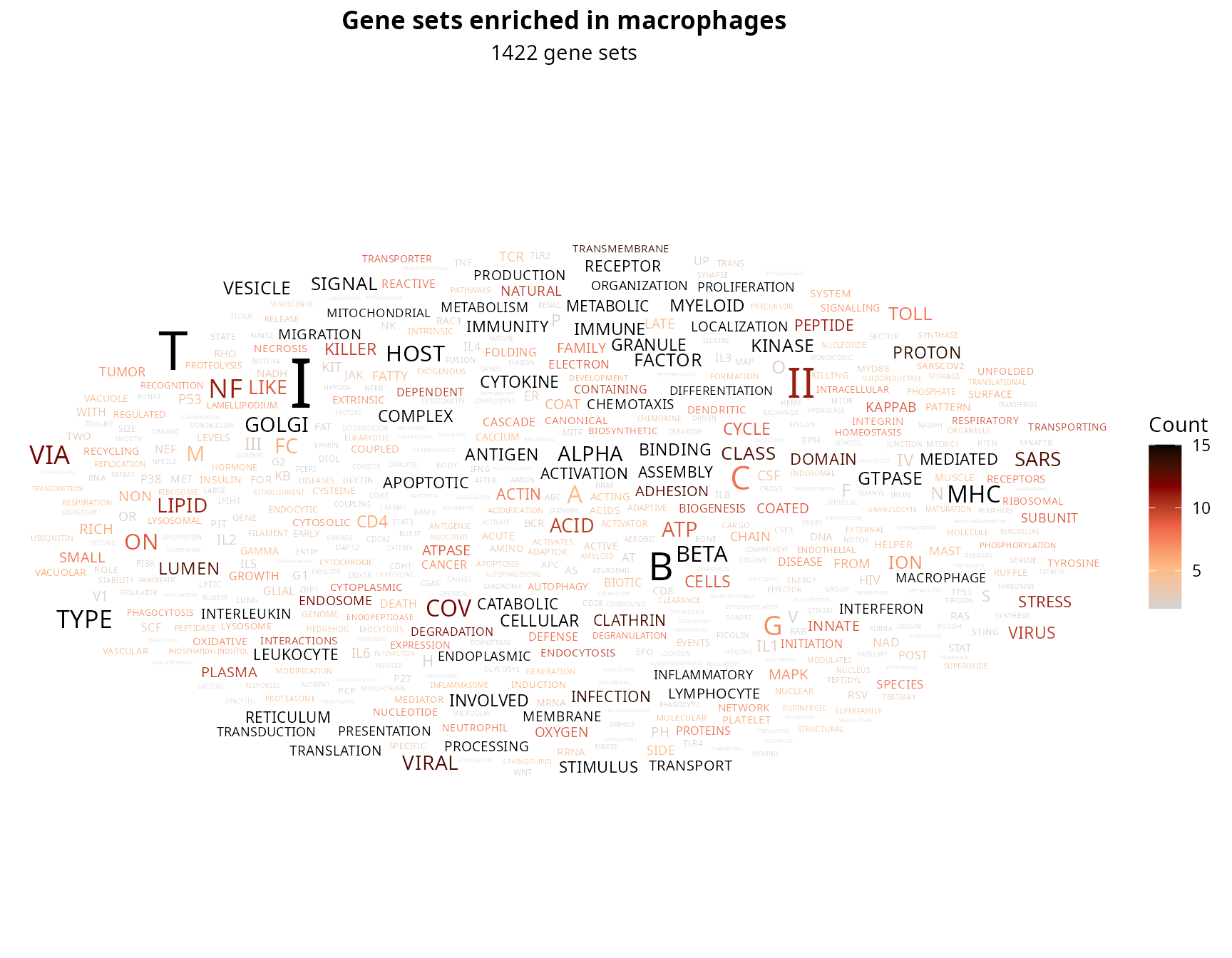
Gene Set Enrichment Analysis
We perform the GSEA by providing a ranked list of genes, order by
their fold change. We compute the fold change using
Seurat’s function. We also add the gene identifiers, as the
GSEA interacts with a database.
df_fold_change = Seurat::FoldChange(sobj,
                                    ident.1 = group1,
                                    ident.2 = group2)

# Add gene ID (gene_corresp and df_fold_change exactly match the gene order)
df_fold_change$ID = gene_corresp$ID
df_fold_change$gene_name = gene_corresp$NAME # not rownames because duplicated are named with .1
rownames(df_fold_change) = gene_corresp$ID

# Fill the table
df_fold_change = df_fold_change %>%
  # Add FC_x_pct
  dplyr::mutate(FC_x_pct = ifelse(avg_log2FC > 0,
                                  yes = avg_log2FC * pct.1,
                                  no = avg_log2FC * pct.2)) %>%
  # Sort
  dplyr::arrange(-avg_log2FC)

head(df_fold_change)
## avg_log2FC pct.1 pct.2 ID gene_name FC_x_pct
## ENSMUSG00000024300 9.246354 0.583 0.000 ENSMUSG00000024300 Myo1f 5.390625
## ENSMUSG00000031165 8.799830 0.501 0.000 ENSMUSG00000031165 Was 4.408715
## ENSMUSG00000022584 8.736281 0.132 0.002 ENSMUSG00000022584 Ly6c2 1.153189
## ENSMUSG00000099974 8.376359 0.299 0.000 ENSMUSG00000099974 Bcl2a1d 2.504531
## ENSMUSG00000053063 8.372347 0.735 0.004 ENSMUSG00000053063 Clec12a 6.153675
## ENSMUSG00000030474 8.326314 0.344 0.000 ENSMUSG00000030474 Siglece 2.864252We define the ranked genes list:
ranked_gene_list = setNames(nm = df_fold_change$ID,
                            df_fold_change$avg_log2FC)
head(ranked_gene_list)
## ENSMUSG00000024300 ENSMUSG00000031165 ENSMUSG00000022584 ENSMUSG00000099974
## 9.246354 8.799830 8.736281 8.376359
## ENSMUSG00000053063 ENSMUSG00000030474
## 8.372347 8.326314Visualization
In this section, we explore various ways to visualize GSEA results.
Barplot
We visualize top 200 gene sets, order by absolute NES, as a barplot:
gsea_results@result %>%
  dplyr::filter(pvalue < 0.05) %>%
  dplyr::top_n(., n = 200, wt = abs(NES)) %>%
  aquarius::plot_gsea_barplot(.,
                              group1 = group1,
                              group2 = group2,
                              nb_char_max = 80)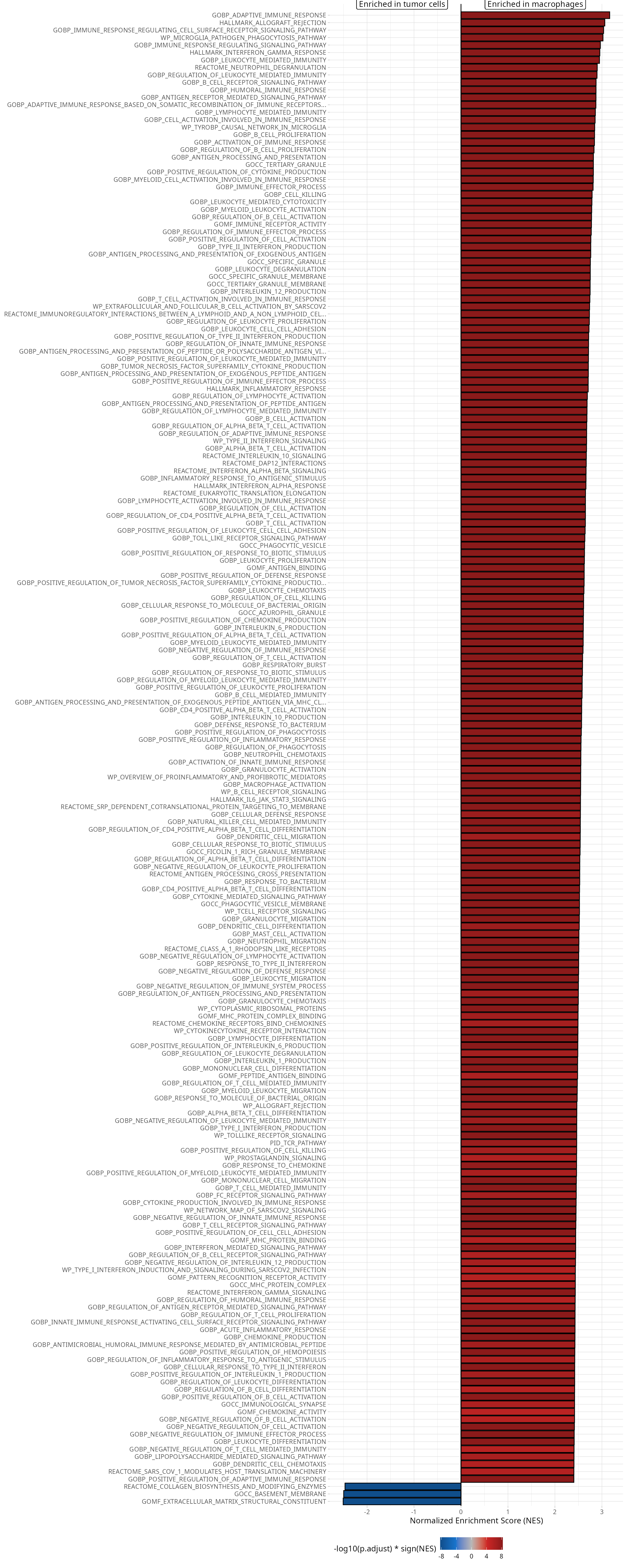
Curve and wordcloud
We make the curve for some gene sets. To easily copy-paste gene set names from the figure, we use:
grep(gsea_results@result$ID,
     pattern = "MATRIX_STRUCT",
     value = TRUE)
## [1] "GOMF_EXTRACELLULAR_MATRIX_STRUCTURAL_CONSTITUENT"
## [2] "GOMF_EXTRACELLULAR_MATRIX_STRUCTURAL_CONSTITUENT_CONFERRING_TENSILE_STRENGTH"
## [3] "GOMF_EXTRACELLULAR_MATRIX_STRUCTURAL_CONSTITUENT_CONFERRING_COMPRESSION_RESISTANCE"
gene_sets_oi = c("GOBP_ADAPTIVE_IMMUNE_RESPONSE",
                 "GOMF_EXTRACELLULAR_MATRIX_STRUCTURAL_CONSTITUENT")

plot_list = lapply(gene_sets_oi, FUN = function(one_gene_set) {
  # Gsea curve
  p = aquarius::plot_gsea_curve(gsea_results,
                                one_gene_set)

  # Wordcloud
  gs_content = gene_sets %>%
    dplyr::filter(gs_name == one_gene_set) %>%
    dplyr::pull(ensembl_gene) %>%
    unique()

  sub_df_fold_change = df_fold_change %>%
    dplyr::filter(ID %in% gs_content)

  p[[4]] = aquarius::plot_wordcloud(sub_df_fold_change,
                                    label = "gene_name",
                                    size_by = "avg_log2FC",
                                    color_by = "FC_x_pct",
                                    max_size = 10)

  # Patchwork
  pp = patchwork::wrap_plots(p,
                             design = "AD\nBD\nCD",
                             widths = c(2, 1.5),
                             heights = c(3, 1, 1))

  return(pp)
})
names(plot_list) = gene_sets_oi

plot_list
## $GOBP_ADAPTIVE_IMMUNE_RESPONSE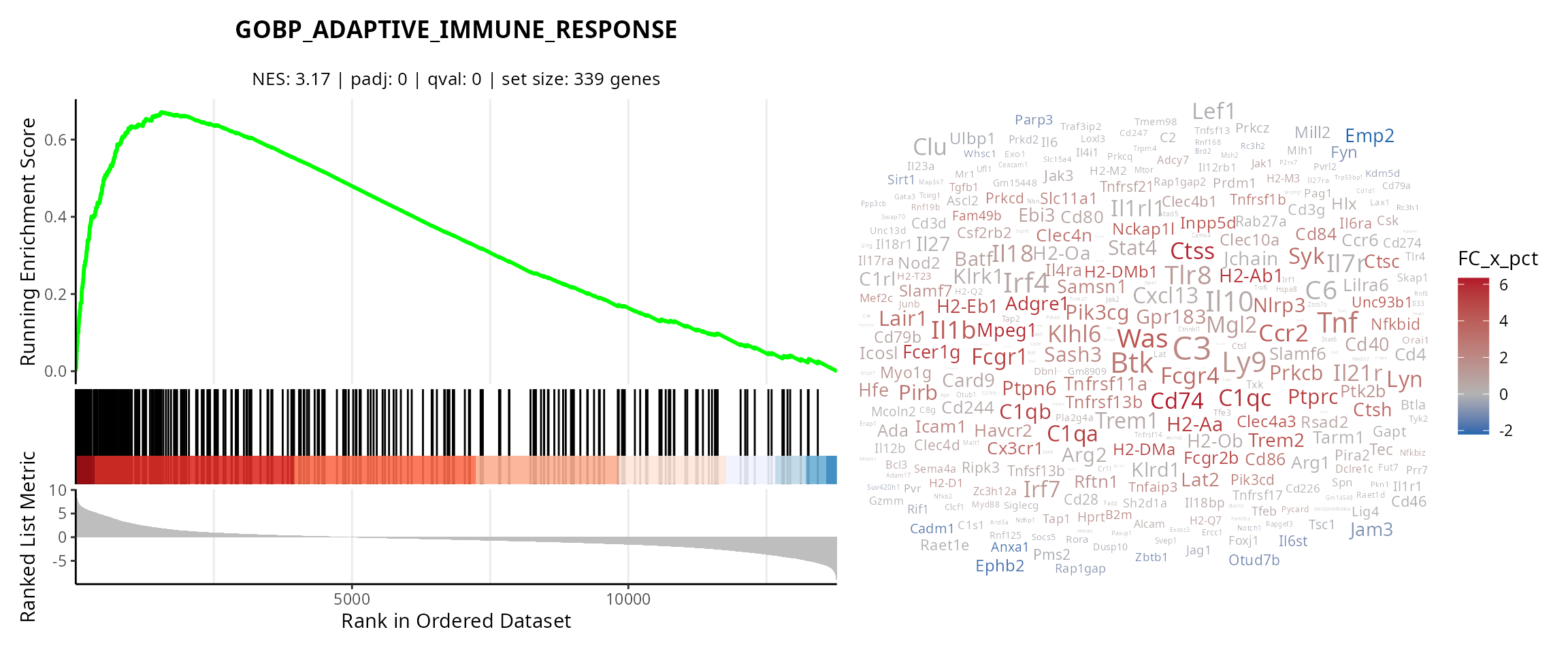
##
## $GOMF_EXTRACELLULAR_MATRIX_STRUCTURAL_CONSTITUENT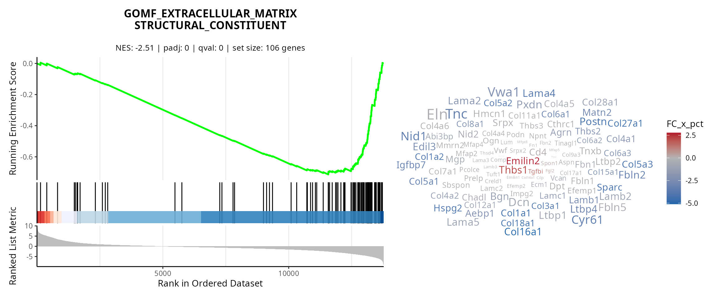
Heatmap
To visualize the evaluate the enrichment at a cellular level and for several gene sets, we make a heatmap depicting cells as columns and gene sets scores as rows.
Gene sets
We filter the enriched gene sets belonging to the HALLMARK category.
hallmark_gene_sets = gene_sets %>%
  dplyr::filter(gs_collection_name == "Hallmark") %>%
  dplyr::pull(gs_name) %>%
  unique()

hallmark_gene_sets
## [1] "HALLMARK_ADIPOGENESIS"
## [2] "HALLMARK_ALLOGRAFT_REJECTION"
## [3] "HALLMARK_ANDROGEN_RESPONSE"
## [4] "HALLMARK_ANGIOGENESIS"
## [5] "HALLMARK_APICAL_JUNCTION"
## [6] "HALLMARK_APICAL_SURFACE"
## [7] "HALLMARK_APOPTOSIS"
## [8] "HALLMARK_BILE_ACID_METABOLISM"
## [9] "HALLMARK_CHOLESTEROL_HOMEOSTASIS"
## [10] "HALLMARK_COAGULATION"
## [11] "HALLMARK_COMPLEMENT"
## [12] "HALLMARK_DNA_REPAIR"
## [13] "HALLMARK_E2F_TARGETS"
## [14] "HALLMARK_EPITHELIAL_MESENCHYMAL_TRANSITION"
## [15] "HALLMARK_ESTROGEN_RESPONSE_EARLY"
## [16] "HALLMARK_ESTROGEN_RESPONSE_LATE"
## [17] "HALLMARK_FATTY_ACID_METABOLISM"
## [18] "HALLMARK_G2M_CHECKPOINT"
## [19] "HALLMARK_GLYCOLYSIS"
## [20] "HALLMARK_HEDGEHOG_SIGNALING"
## [21] "HALLMARK_HEME_METABOLISM"
## [22] "HALLMARK_HYPOXIA"
## [23] "HALLMARK_IL2_STAT5_SIGNALING"
## [24] "HALLMARK_IL6_JAK_STAT3_SIGNALING"
## [25] "HALLMARK_INFLAMMATORY_RESPONSE"
## [26] "HALLMARK_INTERFERON_ALPHA_RESPONSE"
## [27] "HALLMARK_INTERFERON_GAMMA_RESPONSE"
## [28] "HALLMARK_KRAS_SIGNALING_DN"
## [29] "HALLMARK_KRAS_SIGNALING_UP"
## [30] "HALLMARK_MITOTIC_SPINDLE"
## [31] "HALLMARK_MTORC1_SIGNALING"
## [32] "HALLMARK_MYC_TARGETS_V1"
## [33] "HALLMARK_MYC_TARGETS_V2"
## [34] "HALLMARK_MYOGENESIS"
## [35] "HALLMARK_NOTCH_SIGNALING"
## [36] "HALLMARK_OXIDATIVE_PHOSPHORYLATION"
## [37] "HALLMARK_P53_PATHWAY"
## [38] "HALLMARK_PANCREAS_BETA_CELLS"
## [39] "HALLMARK_PEROXISOME"
## [40] "HALLMARK_PI3K_AKT_MTOR_SIGNALING"
## [41] "HALLMARK_PROTEIN_SECRETION"
## [42] "HALLMARK_REACTIVE_OXYGEN_SPECIES_PATHWAY"
## [43] "HALLMARK_SPERMATOGENESIS"
## [44] "HALLMARK_TGF_BETA_SIGNALING"
## [45] "HALLMARK_TNFA_SIGNALING_VIA_NFKB"
## [46] "HALLMARK_UNFOLDED_PROTEIN_RESPONSE"
## [47] "HALLMARK_UV_RESPONSE_DN"
## [48] "HALLMARK_UV_RESPONSE_UP"
## [49] "HALLMARK_WNT_BETA_CATENIN_SIGNALING"
## [50] "HALLMARK_XENOBIOTIC_METABOLISM"We keep only the ones that are enriched in our analysis:
gene_sets_oi = gsea_results@result %>%
  dplyr::filter(ID %in% hallmark_gene_sets) %>%
  dplyr::filter(p.adjust < 0.01) %>%
  dplyr::pull(ID)

gene_sets_oi
## [1] "HALLMARK_ALLOGRAFT_REJECTION"
## [2] "HALLMARK_INTERFERON_GAMMA_RESPONSE"
## [3] "HALLMARK_INFLAMMATORY_RESPONSE"
## [4] "HALLMARK_INTERFERON_ALPHA_RESPONSE"
## [5] "HALLMARK_IL6_JAK_STAT3_SIGNALING"
## [6] "HALLMARK_EPITHELIAL_MESENCHYMAL_TRANSITION"
## [7] "HALLMARK_COMPLEMENT"
## [8] "HALLMARK_TNFA_SIGNALING_VIA_NFKB"
## [9] "HALLMARK_MYOGENESIS"
## [10] "HALLMARK_UV_RESPONSE_DN"
## [11] "HALLMARK_IL2_STAT5_SIGNALING"
## [12] "HALLMARK_PI3K_AKT_MTOR_SIGNALING"
## [13] "HALLMARK_KRAS_SIGNALING_UP"What are the genes in each gene set ?
gene_sets_list = lapply(gene_sets_oi, FUN = function(my_gs_name) {
  gs_content = gene_sets %>%
    dplyr::filter(gs_name == my_gs_name) %>%
    dplyr::pull(ensembl_gene)

  return(gs_content)
})
names(gene_sets_list) = gene_sets_oi

lengths(gene_sets_list)
## HALLMARK_ALLOGRAFT_REJECTION
## 204
## HALLMARK_INTERFERON_GAMMA_RESPONSE
## 209
## HALLMARK_INFLAMMATORY_RESPONSE
## 202
## HALLMARK_INTERFERON_ALPHA_RESPONSE
## 100
## HALLMARK_IL6_JAK_STAT3_SIGNALING
## 89
## HALLMARK_EPITHELIAL_MESENCHYMAL_TRANSITION
## 206
## HALLMARK_COMPLEMENT
## 198
## HALLMARK_TNFA_SIGNALING_VIA_NFKB
## 201
## HALLMARK_MYOGENESIS
## 201
## HALLMARK_UV_RESPONSE_DN
## 144
## HALLMARK_IL2_STAT5_SIGNALING
## 199
## HALLMARK_PI3K_AKT_MTOR_SIGNALING
## 105
## HALLMARK_KRAS_SIGNALING_UP
## 203Score gene sets
We compute scores for each gene set with AUCell. This is
the normalized gene expression matrix:
gene_expression_matrix = sobj@assays[["RNA"]]@layers$data
rownames(gene_expression_matrix) = sobj@assays[["RNA"]]@meta.data$Ensembl_ID
colnames(gene_expression_matrix) = colnames(sobj)

gene_expression_matrix[c(1:5), c(1:3)]
## 5 x 3 sparse Matrix of class "dgCMatrix"
## A_"AAACCCATCAAGTCGT-1" A_"AAAGGTATCGTCTCAC-1"
## ENSMUSG00000051951 . .
## ENSMUSG00000033845 . .
## ENSMUSG00000025903 . .
## ENSMUSG00000033813 . .
## ENSMUSG00000033793 . .
## A_"AAAGTGACATCATTTC-1"
## ENSMUSG00000051951 .
## ENSMUSG00000033845 .
## ENSMUSG00000025903 .
## ENSMUSG00000033813 .
## ENSMUSG00000033793 .(Time to run: 0.02 s)
First, we compute a gene ranking, for all cells and all genes in the dataset.
aucell_rank = AUCell::AUCell_buildRankings(exprMat = gene_expression_matrix,
                                           nCores = n_threads,
                                           plotStats = FALSE)

class(aucell_rank)
## [1] "aucellResults"
## attr(,"package")
## [1] "AUCell"(Time to run: 1.75 s)
We attribute scores for each gene set to each cell, using the gene identifiers to make the connection between our data and the database.
df_scores = AUCell::AUCell_calcAUC(geneSets = gene_sets_list,
                                   rankings = aucell_rank,
                                   nCores = n_threads)
df_scores = AUCell::getAUC(df_scores)

df_scores[c(1:5), c(1:3)]
## cells
## gene sets A_"AAACCCATCAAGTCGT-1"
## HALLMARK_ALLOGRAFT_REJECTION 0.03650220
## HALLMARK_INTERFERON_GAMMA_RESPONSE 0.04777602
## HALLMARK_INFLAMMATORY_RESPONSE 0.03091814
## HALLMARK_INTERFERON_ALPHA_RESPONSE 0.04371403
## HALLMARK_IL6_JAK_STAT3_SIGNALING 0.05922078
## cells
## gene sets A_"AAAGGTATCGTCTCAC-1"
## HALLMARK_ALLOGRAFT_REJECTION 0.11215915
## HALLMARK_INTERFERON_GAMMA_RESPONSE 0.08146097
## HALLMARK_INFLAMMATORY_RESPONSE 0.07587484
## HALLMARK_INTERFERON_ALPHA_RESPONSE 0.07431054
## HALLMARK_IL6_JAK_STAT3_SIGNALING 0.10669331
## cells
## gene sets A_"AAAGTGACATCATTTC-1"
## HALLMARK_ALLOGRAFT_REJECTION 0.10986292
## HALLMARK_INTERFERON_GAMMA_RESPONSE 0.05762131
## HALLMARK_INFLAMMATORY_RESPONSE 0.07687409
## HALLMARK_INTERFERON_ALPHA_RESPONSE 0.04694781
## HALLMARK_IL6_JAK_STAT3_SIGNALING 0.06211788(Time to run: 18.28 s)
(optional) Ordering
On the heatmap, the cells will be ordered by cluster type, then by clusters:
order_CB = sobj@meta.data %>%
  dplyr::arrange(cluster_type, seurat_clusters) %>%
  rownames()

head(order_CB)
## [1] "A_\"AAAGGTATCGTCTCAC-1\"" "A_\"AAAGTGACATCATTTC-1\""
## [3] "A_\"AACAAGAGTTTGATCG-1\"" "A_\"AACACACAGCTTCGTA-1\""
## [5] "A_\"AACCTGAAGGTATTGA-1\"" "A_\"AACTTCTCAGACTGCC-1\""We call this information “pseudotime” and store it in the object:
## A_"AAACCCATCAAGTCGT-1" A_"AAAGGTATCGTCTCAC-1" A_"AAAGTGACATCATTTC-1"
##                    849                      1                      2
## A_"AAAGTGATCATGGAGG-1" A_"AACAAAGTCATTGTTC-1" A_"AACAAGAGTTTGATCG-1"
##                    465                    529                      3
We define a dataframe containing the scores to order and the pseudotime, for each cell:
sobj$cell_CB = colnames(sobj)

## Add a pseudotime column to df_scores
df_features = as.data.frame(t(df_scores)) # cells x features
df_features$cell_CB = rownames(df_features)
df_features = dplyr::left_join(x = df_features,
                               y = sobj@meta.data[, c("cell_CB", "pseudotime")],
                               by = "cell_CB")
df_features$cell_CB = NULL

head(df_features)
## HALLMARK_ALLOGRAFT_REJECTION HALLMARK_INTERFERON_GAMMA_RESPONSE
## 1 0.0365022 0.04777602
## 2 0.1121592 0.08146097
## 3 0.1098629 0.05762131
## 4 0.1204929 0.08311357
## 5 0.1142178 0.16237693
## 6 0.1396942 0.12538678
## HALLMARK_INFLAMMATORY_RESPONSE HALLMARK_INTERFERON_ALPHA_RESPONSE
## 1 0.03091814 0.04371403
## 2 0.07587484 0.07431054
## 3 0.07687409 0.04694781
## 4 0.06249265 0.08077810
## 5 0.10239429 0.17936684
## 6 0.07390572 0.11318220
## HALLMARK_IL6_JAK_STAT3_SIGNALING HALLMARK_EPITHELIAL_MESENCHYMAL_TRANSITION
## 1 0.05922078 0.17467117
## 2 0.10669331 0.06139990
## 3 0.06211788 0.06307494
## 4 0.07462537 0.04060375
## 5 0.05466533 0.02033849
## 6 0.05892108 0.04550073
## HALLMARK_COMPLEMENT HALLMARK_TNFA_SIGNALING_VIA_NFKB HALLMARK_MYOGENESIS
## 1 0.05878251 0.1057509 0.10381961
## 2 0.11884861 0.1754179 0.03478403
## 3 0.11223861 0.1465437 0.02292855
## 4 0.10004952 0.1087483 0.02078783
## 5 0.13226064 0.1634550 0.02160283
## 6 0.13764769 0.1665676 0.02466721
## HALLMARK_UV_RESPONSE_DN HALLMARK_IL2_STAT5_SIGNALING
## 1 0.05557224 0.06270206
## 2 0.01691881 0.04305086
## 3 0.03883820 0.03997713
## 4 0.02865227 0.04756773
## 5 0.03459984 0.08320604
## 6 0.01839704 0.04905774
## HALLMARK_PI3K_AKT_MTOR_SIGNALING HALLMARK_KRAS_SIGNALING_UP pseudotime
## 1 0.05499631 0.05007741 849
## 2 0.08657525 0.07808698 1
## 3 0.06057969 0.08356624 2
## 4 0.10413006 0.06190055 465
## 5 0.07154939 0.08581827 529
## 6 0.07036703 0.06779201 3We identify an order to represent gene sets across clusters.
features_order = aquarius::find_features_order(df_features)

features_order
## [1] "HALLMARK_INTERFERON_ALPHA_RESPONSE"
## [2] "HALLMARK_IL2_STAT5_SIGNALING"
## [3] "HALLMARK_TNFA_SIGNALING_VIA_NFKB"
## [4] "HALLMARK_INTERFERON_GAMMA_RESPONSE"
## [5] "HALLMARK_INFLAMMATORY_RESPONSE"
## [6] "HALLMARK_KRAS_SIGNALING_UP"
## [7] "HALLMARK_PI3K_AKT_MTOR_SIGNALING"
## [8] "HALLMARK_COMPLEMENT"
## [9] "HALLMARK_ALLOGRAFT_REJECTION"
## [10] "HALLMARK_IL6_JAK_STAT3_SIGNALING"
## [11] "HALLMARK_UV_RESPONSE_DN"
## [12] "HALLMARK_MYOGENESIS"
## [13] "HALLMARK_EPITHELIAL_MESENCHYMAL_TRANSITION"(Time to run: 0.85 s)
Preparation
In this section, we prepare the heatmap.
First, we prepare the matrix to build the heatmap without row neither column ordering. To do so :
- Cells are ordered by pseudotime
- Features are ordered as previously defined
- Feature score are normalized between 0 and 1 for each feature, to have blue-to-red scale for each row (feature) in the heatmap
features_order = features_order[features_order %in% rownames(df_scores)]

mat_expression = df_scores[features_order, ]
mat_expression = Matrix::t(mat_expression)
mat_expression = dynutils::scale_quantile(mat_expression) # between 0 and 1
mat_expression = Matrix::t(mat_expression)
dim(mat_expression)
## [1] 13 1108We define custom colors:
list_colors = list()

list_colors[["expression"]] = aquarius::palette_BlWhRd

list_colors[["cell_type"]] = color_markers

list_colors[["clusters"]] = setNames(nm = levels(sobj$seurat_clusters),
                                     aquarius::gg_color_hue(length(levels(sobj$seurat_clusters))))

list_colors[["project_name"]] = setNames(nm = sample_info$project_name,
                                     sample_info$color)

list_colors[["cell_cycle_phase"]] = setNames(nm = c("G0 / G1", "G2M", "S"),
                                             aquarius::gg_color_hue(3))

list_colors[["percent_mito"]] = circlize::colorRamp2(breaks = seq(from = min(sobj$percent.mt),
                                                                  to = max(sobj$percent.mt),
                                                                  length.out = 9),
                                                     colors = RColorBrewer::brewer.pal(name = "Greys", n = 9))

list_colors[["nFeature_RNA"]] = circlize::colorRamp2(breaks = seq(from = min(sobj$nFeature_RNA),
                                                                  to = max(sobj$nFeature_RNA),
                                                                  length.out = 9),
                                                     colors = RColorBrewer::brewer.pal(name = "Greys", n = 9))
We prepare the heatmap annotation:
ha_top = ComplexHeatmap::HeatmapAnnotation(
  group = ComplexHeatmap::anno_block(gp = grid::gpar(fill = list_colors[["cell_type"]]),
                     labels = names(list_colors[["cell_type"]])),
  clusters = sobj$seurat_clusters,
  project_name = sobj$orig.ident,
  col = list(clusters = list_colors[["clusters"]],
             project_name = list_colors[["project_name"]]))

ha_bottom = ComplexHeatmap::HeatmapAnnotation(
  percent_mito = sobj$percent.mt,
  nFeature_RNA = sobj$nFeature_RNA,
  cell_cycle_phase = as.factor(sobj$Seurat.Phase) %>% `levels<-`(c("G0 / G1", "G2M", "S")),
  col = list(percent_mito = list_colors[["percent_mito"]],
             nFeature_RNA = list_colors[["nFeature_RNA"]],
             cell_cycle_phase = list_colors[["cell_cycle_phase"]]))
We build a heatmap:
ht = ComplexHeatmap::Heatmap(
  mat_expression,
  # Expression colors
  col = list_colors[["expression"]],
  heatmap_legend_param = list(title = "expression", at = c(0, 1),
                              labels = c("low", "high")),
  # Annotation
  top_annotation = ha_top,
  bottom_annotation = ha_bottom,
  # Cells grouping
  column_split = sobj$cluster_type,
  column_gap = unit(2, "mm"),
  column_title = NULL,
  # Cells order
  column_order = match(order_CB, colnames(sobj)),
  cluster_columns = FALSE,
  # Cells label
  show_column_names = FALSE,
  # Gene grouping
  row_order = features_order,
  cluster_rows = FALSE,
  # Gene labels
  show_row_names = TRUE,
  row_names_gp = grid::gpar(fontsize = 12),
  # Visual aspect
  show_heatmap_legend = TRUE,
  border = TRUE,
  use_raster = FALSE)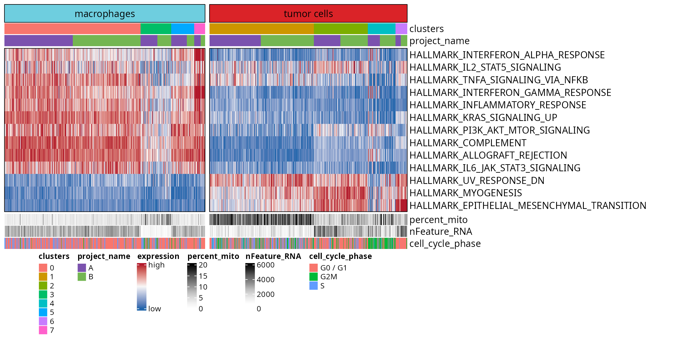
Save
The list_results looks like:
names(list_results)## [1] "macrophages_vs_tumor cells"
names(list_results[[1]])## [1] "de" "up" "gsea"
lapply(list_results[[1]], FUN = class)## $de
## [1] "data.frame"
##
## $up
## [1] "list"
##
## $gsea
## [1] "gseaResult"
## attr(,"package")
## [1] "DOSE"We save the list_results
(eval = FALSE):
R Session
show
## R version 4.4.3 (2025-02-28)
## Platform: x86_64-pc-linux-gnu
## Running under: Ubuntu 24.10
##
## Matrix products: default
## BLAS:   /usr/lib/x86_64-linux-gnu/blas/libblas.so.3.12.0
## LAPACK: /usr/lib/x86_64-linux-gnu/lapack/liblapack.so.3.12.0
##
## locale:
##  [1] LC_CTYPE=en_US.UTF-8       LC_NUMERIC=C
##  [3] LC_TIME=fr_FR.UTF-8        LC_COLLATE=en_US.UTF-8
##  [5] LC_MONETARY=fr_FR.UTF-8    LC_MESSAGES=en_US.UTF-8
##  [7] LC_PAPER=fr_FR.UTF-8       LC_NAME=C
##  [9] LC_ADDRESS=C               LC_TELEPHONE=C
## [11] LC_MEASUREMENT=fr_FR.UTF-8 LC_IDENTIFICATION=C
##
## time zone: Europe/Paris
## tzcode source: system (glibc)
##
## attached base packages:
## [1] stats     graphics  grDevices utils     datasets  methods   base
##
## other attached packages:
## [1] ggplot2_3.5.2   patchwork_1.3.0 dplyr_1.1.4
##
## loaded via a namespace (and not attached):
##   [1] ggtext_0.1.2                fs_1.6.6
##   [3] matrixStats_1.5.0           spatstat.sparse_3.1-0
##   [5] enrichplot_1.26.6           httr_1.4.7
##   [7] RColorBrewer_1.1-3          doParallel_1.0.17
##   [9] tools_4.4.3                 sctransform_0.4.2
##  [11] R6_2.6.1                    lazyeval_0.2.2
##  [13] uwot_0.2.3                  GetoptLong_1.0.5
##  [15] litedown_0.7                withr_3.0.2
##  [17] sp_2.2-0                    gridExtra_2.3
##  [19] progressr_0.15.1            cli_3.6.5
##  [21] Biobase_2.66.0              textshaping_1.0.1
##  [23] Cairo_1.6-2                 aquarius_1.0.0
##  [25] spatstat.explore_3.4-2      fastDummies_1.7.5
##  [27] labeling_0.4.3              sass_0.4.10
##  [29] Seurat_5.3.0                spatstat.data_3.1-6
##  [31] readr_2.1.5                 ggridges_0.5.6
##  [33] pbapply_1.7-2               pkgdown_2.1.2
##  [35] systemfonts_1.2.3           commonmark_1.9.5
##  [37] yulab.utils_0.2.0           gson_0.1.0
##  [39] DOSE_4.0.1                  R.utils_2.13.0
##  [41] parallelly_1.43.0           limma_3.62.2
##  [43] RSQLite_2.3.10              gridGraphics_0.5-1
##  [45] generics_0.1.3              shape_1.4.6.1
##  [47] ica_1.0-3                   spatstat.random_3.3-3
##  [49] GO.db_3.20.0                Matrix_1.7-3
##  [51] S4Vectors_0.44.0            abind_1.4-8
##  [53] R.methodsS3_1.8.2           lifecycle_1.0.4
##  [55] yaml_2.3.10                 SummarizedExperiment_1.36.0
##  [57] qvalue_2.38.0               SparseArray_1.6.2
##  [59] Rtsne_0.17                  grid_4.4.3
##  [61] blob_1.2.4                  promises_1.3.2
##  [63] crayon_1.5.3                ggtangle_0.0.6
##  [65] miniUI_0.1.2                lattice_0.22-6
##  [67] msigdbr_10.0.2              cowplot_1.1.3
##  [69] annotate_1.84.0             KEGGREST_1.46.0
##  [71] pillar_1.10.2               knitr_1.50
##  [73] ComplexHeatmap_2.23.1       fgsea_1.32.4
##  [75] GenomicRanges_1.58.0        rjson_0.2.23
##  [77] future.apply_1.11.3         codetools_0.2-20
##  [79] fastmatch_1.1-6             glue_1.8.0
##  [81] ggfun_0.1.8                 spatstat.univar_3.1-2
##  [83] remotes_2.5.0               data.table_1.17.0
##  [85] treeio_1.30.0               vctrs_0.6.5
##  [87] png_0.1-8                   spam_2.11-1
##  [89] org.Mm.eg.db_3.20.0         gtable_0.3.6
##  [91] assertthat_0.2.1            cachem_1.1.0
##  [93] xfun_0.52                   S4Arrays_1.6.0
##  [95] mime_0.13                   survival_3.8-3
##  [97] SingleCellExperiment_1.28.1 iterators_1.0.14
##  [99] statmod_1.5.0               fitdistrplus_1.2-2
## [101] ROCR_1.0-11                 nlme_3.1-168
## [103] dynutils_1.0.11             doMC_1.3.8
## [105] ggtree_3.14.0               bit64_4.6.0-1
## [107] RcppAnnoy_0.0.22            GenomeInfoDb_1.42.3
## [109] ggwordcloud_0.6.2           bslib_0.9.0
## [111] irlba_2.3.5.1               KernSmooth_2.23-26
## [113] colorspace_2.1-1            BiocGenerics_0.52.0
## [115] DBI_1.2.3                   tidyselect_1.2.1
## [117] proxyC_0.5.2                AUCell_1.28.0
## [119] bit_4.6.0                   compiler_4.4.3
## [121] graph_1.84.1                xml2_1.3.8
## [123] desc_1.4.3                  DelayedArray_0.32.0
## [125] plotly_4.10.4               msigdbdf_24.1.1
## [127] scales_1.4.0                lmtest_0.9-40
## [129] stringr_1.5.1               digest_0.6.37
## [131] goftest_1.2-3               spatstat.utils_3.1-3
## [133] rmarkdown_2.29              XVector_0.46.0
## [135] htmltools_0.5.8.1           pkgconfig_2.0.3
## [137] sparseMatrixStats_1.18.0    MatrixGenerics_1.18.1
## [139] fastmap_1.2.0               rlang_1.1.6
## [141] GlobalOptions_0.1.2         htmlwidgets_1.6.4
## [143] UCSC.utils_1.2.0            DelayedMatrixStats_1.28.1
## [145] shiny_1.10.0                farver_2.1.2
## [147] jquerylib_0.1.4             zoo_1.8-14
## [149] jsonlite_2.0.0              BiocParallel_1.40.2
## [151] GOSemSim_2.32.0             R.oo_1.27.1
## [153] magrittr_2.0.3              ggplotify_0.1.2
## [155] GenomeInfoDbData_1.2.13     dotCall64_1.2
## [157] Rcpp_1.0.14                 ape_5.8-1
## [159] babelgene_22.9              reticulate_1.42.0
## [161] stringi_1.8.7               ggalluvial_0.12.5
## [163] zlibbioc_1.52.0             MASS_7.3-65
## [165] plyr_1.8.9                  parallel_4.4.3
## [167] listenv_0.9.1               ggrepel_0.9.6
## [169] deldir_2.0-4                Biostrings_2.74.1
## [171] splines_4.4.3               gridtext_0.1.5
## [173] tensor_1.5                  hms_1.1.3
## [175] circlize_0.4.16             igraph_2.1.4
## [177] spatstat.geom_3.3-6         markdown_2.0
## [179] RcppHNSW_0.6.0              reshape2_1.4.4
## [181] stats4_4.4.3                XML_3.99-0.18
## [183] evaluate_1.0.3              SeuratObject_5.1.0
## [185] tzdb_0.5.0                  foreach_1.5.2
## [187] httpuv_1.6.16               RANN_2.6.2
## [189] tidyr_1.3.1                 purrr_1.0.4
## [191] polyclip_1.10-7             future_1.40.0
## [193] clue_0.3-66                 scattermore_1.2
## [195] xtable_1.8-4                tidytree_0.4.6
## [197] RSpectra_0.16-2             later_1.4.2
## [199] viridisLite_0.4.2           ragg_1.4.0
## [201] tibble_3.2.1                clusterProfiler_4.14.6
## [203] aplot_0.2.5                 memoise_2.0.1
## [205] AnnotationDbi_1.68.0        IRanges_2.40.1
## [207] cluster_2.1.8.1             globals_0.17.0
## [209] GSEABase_1.68.0