Quality control
Sample A
2025-05-03
Source:vignettes/examples/1_individual/1_qc_annotation.Rmd
1_qc_annotation.RmdThis notebook shows the use of these functions from
aquarius:
aquarius::create_parallel_instanceaquarius::load_sc_dataaquarius::cell_annot_customaquarius::add_cell_cycleaquarius::find_doubletsaquarius::plot_dfaquarius::plot_dotplotaquarius::plot_barplotaquarius::plot_qc_densityaquarius::plot_qc_facslikeaquarius::plot_piechartaquarius::plot_doublets_compositionaquarius::palette_GrOrBlaquarius::gg_color_hue
The goal of this script is to generate a Seurat object from the raw count matrix for sample A.
## [1] "/usr/lib/R/library"            "/usr/local/lib/R/site-library"
## [3] "/usr/lib/R/site-library"
Preparation
In this section, we set the global settings of the analysis. We will store data there:
out_dir = "."

if (!dir.exists(paste0(out_dir, "/datasets/"))) {
  dir.create(paste0(out_dir, "/datasets/"), recursive = TRUE)
}
We load the parameters:
sample_name = params$sample_nameInput count matrix is there:
count_matrix_dir = system.file(paste0("extdata/", sample_name, "/"),
                               package = "aquarius")

list.files(count_matrix_dir)
## [1] "barcodes.tsv.gz" "features.tsv.gz" "matrix.mtx.gz"We load the markers and specific colors for each cell type:
cell_markers = list("macrophages" = c("Ptprc", "Adgre1", "Lcp1", "Aif1", "Fcgr3"),
                    "tumor cells" = c("Sox9", "Sox10", "Ank3", "Plp1", "Col16a1"))

lengths(cell_markers)
## macrophages tumor cells
## 5 5Here are custom colors for each cell type:
color_markers = c("macrophages" = "#6ECEDF",
                  "tumor cells" = "#DA2328")
We define markers to display on the dotplot:
We define custom colors for each sample:
sample_info = data.frame(
  project_name = c("A", "B"),
  sample_identifier = c("A", "B"),
  color = c("#7B52AE", "#74B652"),
  row.names = c("A", "B"))

aquarius::plot_df(sample_info)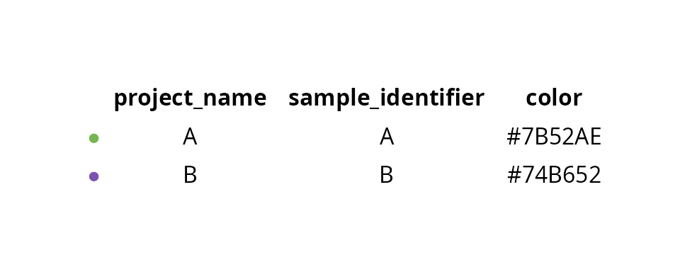
We set main parameters:
n_threads = 10L
cl = aquarius::create_parallel_instance(nthreads = n_threads)
num_threads = n_threads # Rtsne::Rtsne option

cut_log_nCount_RNA = 6
cut_nFeature_RNA = 600
cut_percent.mt = 20
cut_percent.rb = 20

ndims = 20
Load count matrix
In this section, we load the raw count matrix. The function further estimates and applies a filtering of empty droplets.
sobj = aquarius::load_sc_data(data_path = count_matrix_dir,
                              sample_name = sample_name,
                              BPPARAM = cl)
sobj
## An object of class Seurat
## 28000 features across 817 samples within 1 assay
## Active assay: RNA (28000 features, 0 variable features)
## 1 layer present: countsIn genes metadata, we add the Ensembl ID. The
sobj@assays$RNA@meta.data dataframe contains three
information:
-
rownames: gene names stored as the “dimnames” of the count matrix. Duplicated gene names will have a “.1” at the end of their name -
Ensembl_ID: Ensembl ID, as stored in thefeatures.tsv.gzfile -
gene_name: gene name, as stored in thefeatures.tsv.gzfile. Duplicated gene names will have the same name.
features_df = read.csv(paste0(count_matrix_dir, "/features.tsv.gz"), sep = "\t", header = 0)
features_df = features_df[, c(1:2)]
colnames(features_df) = c("Ensembl_ID", "gene_name")
rownames(features_df) = rownames(sobj) # mandatory for Seurat::FindVariableFeatures

sobj@assays$RNA@meta.data = features_df
rm(features_df)

head(sobj@assays$RNA@meta.data)
## Ensembl_ID gene_name
## Xkr4 ENSMUSG00000051951 Xkr4
## Gm1992 ENSMUSG00000089699 Gm1992
## Gm37381 ENSMUSG00000102343 Gm37381
## Rp1 ENSMUSG00000025900 Rp1
## Rp1.1 ENSMUSG00000109048 Rp1
## Sox17 ENSMUSG00000025902 Sox17
summary(sobj@meta.data)## orig.ident nCount_RNA nFeature_RNA log_nCount_RNA
## A:817 Min. : 106 Min. : 92 Min. : 4.663
## 1st Qu.: 1965 1st Qu.: 924 1st Qu.: 7.583
## Median : 5299 Median :1924 Median : 8.575
## Mean : 7229 Mean :2105 Mean : 8.333
## 3rd Qu.:11002 3rd Qu.:3066 3rd Qu.: 9.306
## Max. :56790 Max. :7097 Max. :10.947Processing
Gene expression normalization
We normalize the count matrix and identity the most variable features.
sobj = Seurat::NormalizeData(sobj,
                             normalization.method = "LogNormalize",
                             assay = "RNA")

sobj = Seurat::FindVariableFeatures(sobj,
                                    assay = "RNA",
                                    nfeatures = 3000)
sobj
## An object of class Seurat
## 28000 features across 817 samples within 1 assay
## Active assay: RNA (28000 features, 3000 variable features)
## 2 layers present: counts, dataProjection
We generate a tSNE to visualize cells before filtering. Prior to this, we build a PCA from the scaled normalized matrix of highly variable genes.
sobj = Seurat::ScaleData(sobj)
sobj = Seurat::RunPCA(sobj,
                      assay = "RNA",
                      reduction.name = "RNA_pca",
                      npcs = 100)

Seurat::ElbowPlot(sobj, ndims = 100, reduction = "RNA_pca")
We generate a tSNE with 20 principal components:
sobj = Seurat::RunTSNE(sobj,
                       reduction = "RNA_pca",
                       dims = 1:ndims,
                       seed.use = 1337L,
                       reduction.name = paste0("RNA_pca_", ndims, "_tsne"),
                       num_threads = num_threads)

sobj
## An object of class Seurat
## 28000 features across 817 samples within 1 assay
## Active assay: RNA (28000 features, 3000 variable features)
## 3 layers present: counts, data, scale.data
## 2 dimensional reductions calculated: RNA_pca, RNA_pca_20_tsneAnnotation
Cell type
We annotate cells for cell type using a modified version of the
Seurat::AddModuleScore function.
sobj = aquarius::cell_annot_custom(sobj,
                                   newname = "cell_type",
                                   markers = cell_markers,
                                   use_negative = TRUE,
                                   add_score = TRUE)

table(sobj$cell_type)
##
## macrophages tumor cells
## 413 404To justify cell type annotation, we can make a dotplot:
aquarius::plot_dotplot(sobj, assay = "RNA",
                       column_name = "cell_type",
                       markers = dotplot_markers,
                       nb_hline = 0) +
  ggplot2::scale_color_gradientn(colors = aquarius::palette_GrOrBl) +
  ggplot2::theme(legend.position = "right",
                 legend.box = "vertical",
                 legend.direction = "vertical",
                 axis.title = element_blank(),
                 axis.text = element_text(size = 15))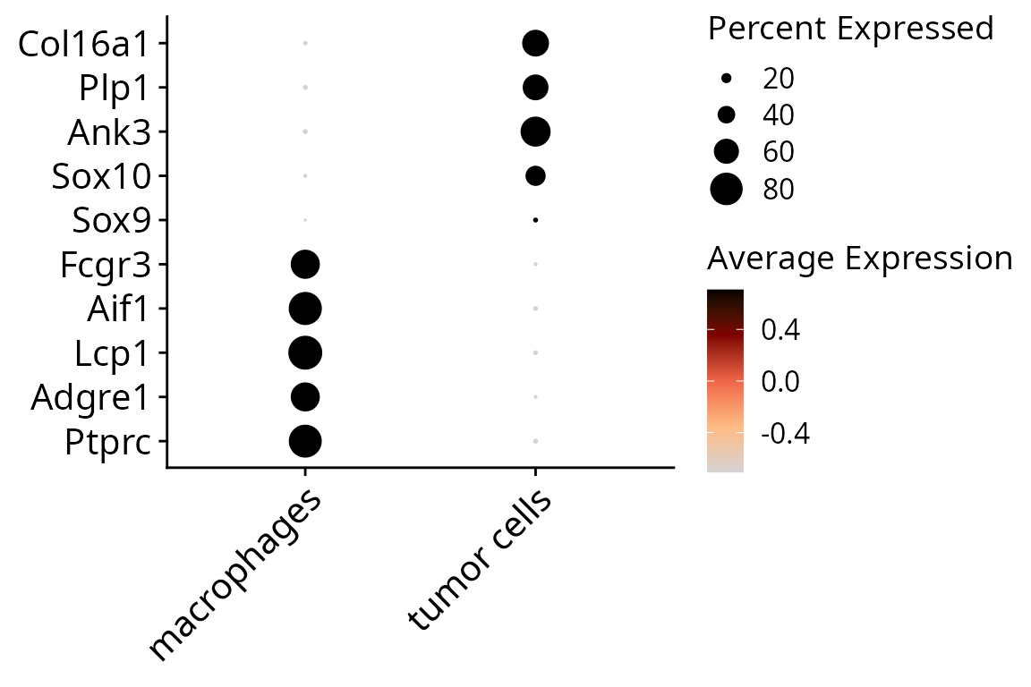
We can make a barplot to see the composition of each dataset, and visualize cell types on the projection.
df_proportion = as.data.frame(prop.table(table(sobj$orig.ident,
                                               sobj$cell_type)))
colnames(df_proportion) = c("orig.ident", "cell_type", "freq")

quantif = table(sobj$orig.ident) %>%
  as.data.frame.table() %>%
  `colnames<-`(c("orig.ident", "nb_cells"))

# Plot
plot_list = list()

plot_list[[2]] = aquarius::plot_barplot(df = df_proportion,
                                        x = "orig.ident",
                                        y = "freq",
                                        fill = "cell_type",
                                        position = ggplot2::position_fill()) +
  ggplot2::scale_fill_manual(name = "Cell type",
                             values = color_markers[levels(df_proportion$cell_type)],
                             breaks = levels(df_proportion$cell_type)) +
  ggplot2::geom_label(data = quantif, inherit.aes = FALSE,
                      aes(x = orig.ident, y = 1.05, label = nb_cells),
                      label.size = 0)

plot_list[[1]] = Seurat::DimPlot(sobj, group.by = "cell_type",
                                 reduction = paste0("RNA_pca_", ndims, "_tsne")) +
  ggplot2::scale_color_manual(values = unlist(color_markers),
                              breaks = names(color_markers)) +
  ggplot2::labs(title = sample_name,
                subtitle = paste0(ncol(sobj), " cells")) +
  Seurat::NoLegend() + Seurat::NoAxes() +
  ggplot2::theme(aspect.ratio = 1,
                 plot.title = element_text(hjust = 0.5),
                 plot.subtitle = element_text(hjust = 0.5))

patchwork::wrap_plots(plot_list, nrow = 1, widths = c(6, 1))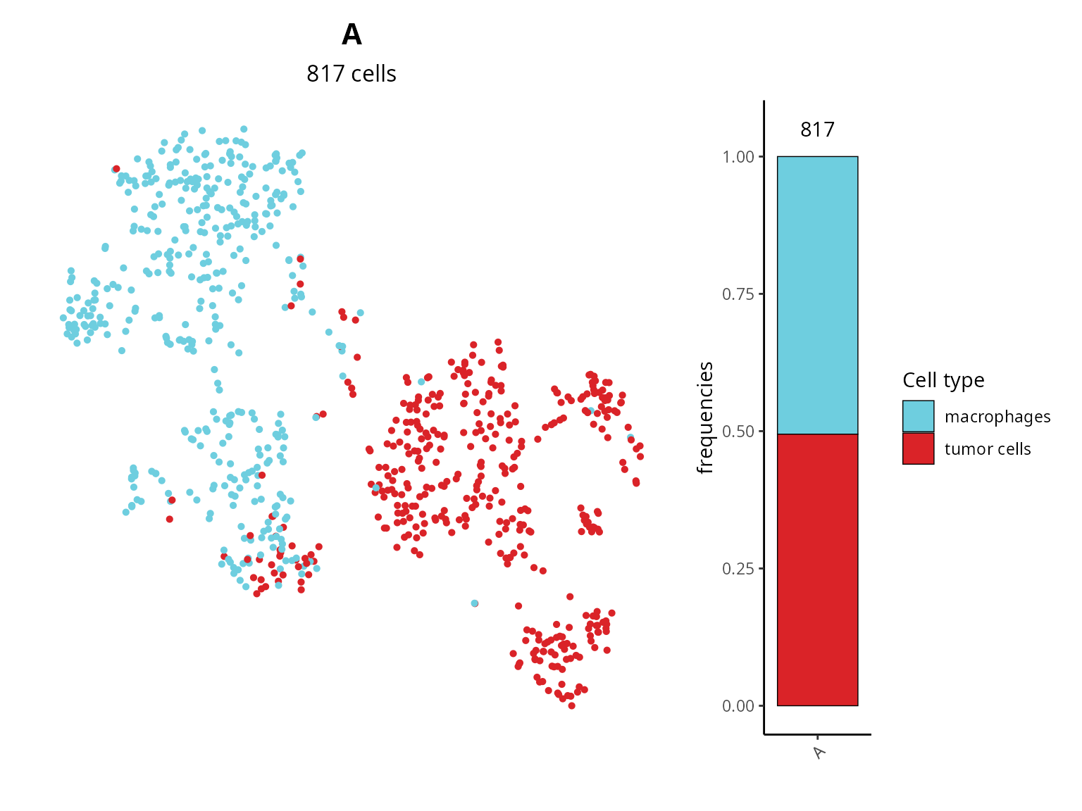
Cell cycle
We annotate cells for cell cycle phase using Seurat and
cyclone.
cc_columns = aquarius::add_cell_cycle(sobj = sobj,
                                      assay = "RNA",
                                      species_rdx = "mm",
                                      BPPARAM = cl)@meta.data[, c("Seurat.Phase", "Phase")]

sobj$Seurat.Phase = cc_columns$Seurat.Phase
sobj$cyclone.Phase = cc_columns$Phase

table(sobj$Seurat.Phase, sobj$cyclone.Phase)
##
## G1 G2M S
## G1 426 13 3
## G2M 124 44 4
## S 193 6 1We visualize cell cycle on the projection:
plot_list = list()

plot_list[[2]] = Seurat::DimPlot(sobj, group.by = "Seurat.Phase",
                                 reduction = paste0("RNA_pca_", ndims, "_tsne")) +
  ggplot2::labs(title = "Cell Cycle Phase",
                subtitle = "Seurat.Phase") +
  Seurat::NoLegend() + Seurat::NoAxes() +
  ggplot2::theme(aspect.ratio = 1,
                 plot.title = element_text(hjust = 0.5),
                 plot.subtitle = element_text(hjust = 0.5))

plot_list[[1]] = Seurat::DimPlot(sobj, group.by = "cyclone.Phase",
                                 reduction = paste0("RNA_pca_", ndims, "_tsne")) +
  ggplot2::labs(title = "Cell Cycle Phase",
                subtitle = "cyclone.Phase") +
  Seurat::NoLegend() + Seurat::NoAxes() +
  ggplot2::theme(aspect.ratio = 1,
                 plot.title = element_text(hjust = 0.5),
                 plot.subtitle = element_text(hjust = 0.5))

patchwork::wrap_plots(plot_list, nrow = 1)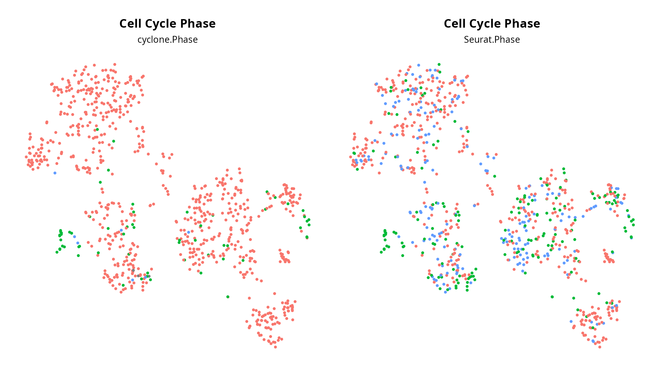
Clustering
We make a clustering:
sobj = Seurat::FindNeighbors(sobj, reduction = "RNA_pca", dims = c(1:ndims))
sobj = Seurat::FindClusters(sobj, resolution = 0.5)
## Modularity Optimizer version 1.3.0 by Ludo Waltman and Nees Jan van Eck
##
## Number of nodes: 817
## Number of edges: 25258
##
## Running Louvain algorithm...
## Maximum modularity in 10 random starts: 0.8551
## Number of communities: 8
## Elapsed time: 0 seconds
table(sobj$seurat_clusters)##
## 0 1 2 3 4 5 6 7
## 232 226 145 82 52 50 16 14We visualize the clustering:
Seurat::DimPlot(sobj, group.by = "seurat_clusters", label = TRUE,
                reduction = paste0("RNA_pca_", ndims, "_tsne")) +
  Seurat::NoAxes() + ggplot2::ggtitle("tSNE") +
  ggplot2::theme(aspect.ratio = 1,
                 plot.title = element_text(hjust = 0.5),
                 legend.position = "none")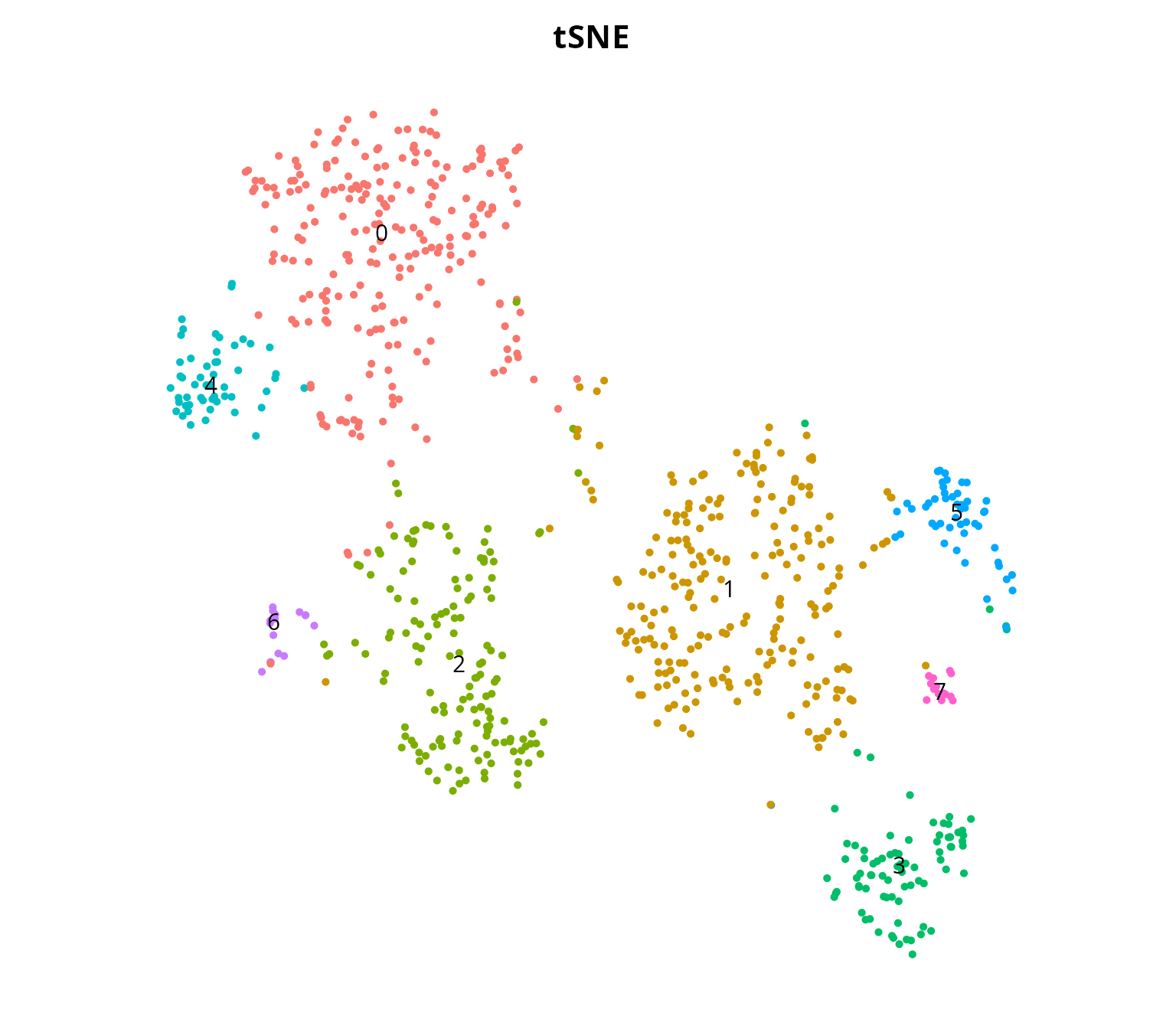
Quality control
In this section, we look at the number of genes expressed by each cell, the number of UMI, the percentage of mitochondrial genes expressed, and the percentage of ribosomal genes expressed. Then, without taking into account the cells expressing low number of genes or have low number of UMI, we identify doublet cells.
The goal is next to filter cells:
- cells with a number of UMI lower than 6
- cells expressing a number of genes lower than 600
- cells having more than 20 % of UMI related to mitochondrial genes
- cells having more than 20 % of UMI related to ribosomal genes
- doublet cells detected with both methods (union of scDblFinder and scds-hybrid)
First, we add the columns associated with the percentage of UMI related to mitochondrial genes or ribosomal genes.
sobj = Seurat::PercentageFeatureSet(sobj, pattern = "^mt", col.name = "percent.mt")
sobj = Seurat::PercentageFeatureSet(sobj, pattern = "^Rp[l|s][0-9]*$", col.name = "percent.rb")

head(sobj@meta.data)
## orig.ident nCount_RNA nFeature_RNA log_nCount_RNA
## "AAACCCATCAAGTCGT-1" A 6183 2815 8.729559
## "AAAGGTATCGTCTCAC-1" A 5226 1669 8.561401
## "AAAGTCCGTTGTACGT-1" A 5985 1307 8.697012
## "AAAGTGACATCATTTC-1" A 4302 2008 8.366835
## "AAAGTGATCATGGAGG-1" A 5350 1987 8.584852
## "AACAAAGCAAGTGGAC-1" A 10390 1871 9.248599
## score_macrophages score_tumor_cells cell_type
## "AAACCCATCAAGTCGT-1" -1.232917651 1.1494669 tumor cells
## "AAAGGTATCGTCTCAC-1" 1.047019910 -0.7155429 macrophages
## "AAAGTCCGTTGTACGT-1" -0.739745937 -0.6703637 macrophages
## "AAAGTGACATCATTTC-1" 0.983434788 -0.7969395 macrophages
## "AAAGTGATCATGGAGG-1" 0.002740319 -0.7714659 macrophages
## "AACAAAGCAAGTGGAC-1" -1.045713950 -0.5272919 tumor cells
## Seurat.Phase cyclone.Phase RNA_snn_res.0.5 seurat_clusters
## "AAACCCATCAAGTCGT-1" G1 G1 3 3
## "AAAGGTATCGTCTCAC-1" S G1 0 0
## "AAAGTCCGTTGTACGT-1" G2M G1 5 5
## "AAAGTGACATCATTTC-1" S G1 0 0
## "AAAGTGATCATGGAGG-1" G1 G1 4 4
## "AACAAAGCAAGTGGAC-1" G2M G1 5 5
## percent.mt percent.rb
## "AAACCCATCAAGTCGT-1" 4.075691 4.657933
## "AAAGGTATCGTCTCAC-1" 2.525832 7.462687
## "AAAGTCCGTTGTACGT-1" 5.480368 35.271512
## "AAAGTGACATCATTTC-1" 1.859600 4.788470
## "AAAGTGATCATGGAGG-1" 6.317757 10.242991
## "AACAAAGCAAGTGGAC-1" 6.381136 26.737247We get the cell barcodes for the failing cells:
fail_percent.mt = sobj@meta.data %>% dplyr::filter(percent.mt > cut_percent.mt) %>% rownames()
fail_percent.rb = sobj@meta.data %>% dplyr::filter(percent.rb > cut_percent.rb) %>% rownames()
fail_log_nCount_RNA = sobj@meta.data %>% dplyr::filter(log_nCount_RNA < cut_log_nCount_RNA) %>% rownames()
fail_nFeature_RNA = sobj@meta.data %>% dplyr::filter(nFeature_RNA < cut_nFeature_RNA) %>% rownames()
Doublet cells detection
Without taking into account the cells with low number of UMI or genes, we identify doublets. First, we filter the Seurat object for the “almost empty” cells.
fsobj = subset(sobj, invert = TRUE,
               cells = unique(c(fail_log_nCount_RNA, fail_nFeature_RNA)))
fsobj
## An object of class Seurat
## 28000 features across 700 samples within 1 assay
## Active assay: RNA (28000 features, 3000 variable features)
## 3 layers present: counts, data, scale.data
## 2 dimensional reductions calculated: RNA_pca, RNA_pca_20_tsneOn this filtered dataset, we apply doublet cells detection. Just before, we run the normalization, taking into account only the remaining cells.
fsobj = Seurat::NormalizeData(fsobj,
                              normalization.method = "LogNormalize",
                              assay = "RNA")

fsobj = Seurat::FindVariableFeatures(fsobj,
                                     assay = "RNA",
                                     nfeatures = 3000)
fsobj
## An object of class Seurat
## 28000 features across 700 samples within 1 assay
## Active assay: RNA (28000 features, 3000 variable features)
## 3 layers present: counts, data, scale.data
## 2 dimensional reductions calculated: RNA_pca, RNA_pca_20_tsneWe identify doublet cells:
fsobj = aquarius::find_doublets(sobj = fsobj,
                                BPPARAM = cl)

fail_doublets_consensus = Seurat::WhichCells(fsobj, expression = doublets_consensus.class)
fail_doublets_scDblFinder = Seurat::WhichCells(fsobj, expression = scDblFinder.class)
fail_doublets_hybrid = Seurat::WhichCells(fsobj, expression = hybrid_score.class)
We add the information in the non filtered Seurat object:
sobj$doublets_consensus.class = dplyr::case_when(!(colnames(sobj) %in% colnames(fsobj)) ~ NA,
                                                 colnames(sobj) %in% fail_doublets_consensus ~ TRUE,
                                                 !(colnames(sobj) %in% fail_doublets_consensus) ~ FALSE)

sobj$scDblFinder.class = dplyr::case_when(!(colnames(sobj) %in% colnames(fsobj)) ~ NA,
                                          colnames(sobj) %in% fail_doublets_scDblFinder ~ TRUE,
                                          !(colnames(sobj) %in% fail_doublets_scDblFinder) ~ FALSE)

sobj$hybrid_score.class = dplyr::case_when(!(colnames(sobj) %in% colnames(fsobj)) ~ NA,
                                           colnames(sobj) %in% fail_doublets_hybrid ~ TRUE,
                                           !(colnames(sobj) %in% fail_doublets_hybrid) ~ FALSE)
Quality control representation
We visualize the four quality metrics:
plot_list = lapply(c("nFeature_RNA", "log_nCount_RNA",
                     "percent.mt", "percent.rb"), FUN = function(one_metric) {
                       p = Seurat::FeaturePlot(sobj, features = one_metric,
                                               reduction = paste0("RNA_pca_", ndims, "_tsne")) +
                         ggplot2::scale_color_gradientn(colors = aquarius::palette_GrOrBl) +
                         ggplot2::theme(aspect.ratio = 1) +
                         Seurat::NoAxes()
                       return(p)
                     })

patchwork::wrap_plots(plot_list, ncol = 4)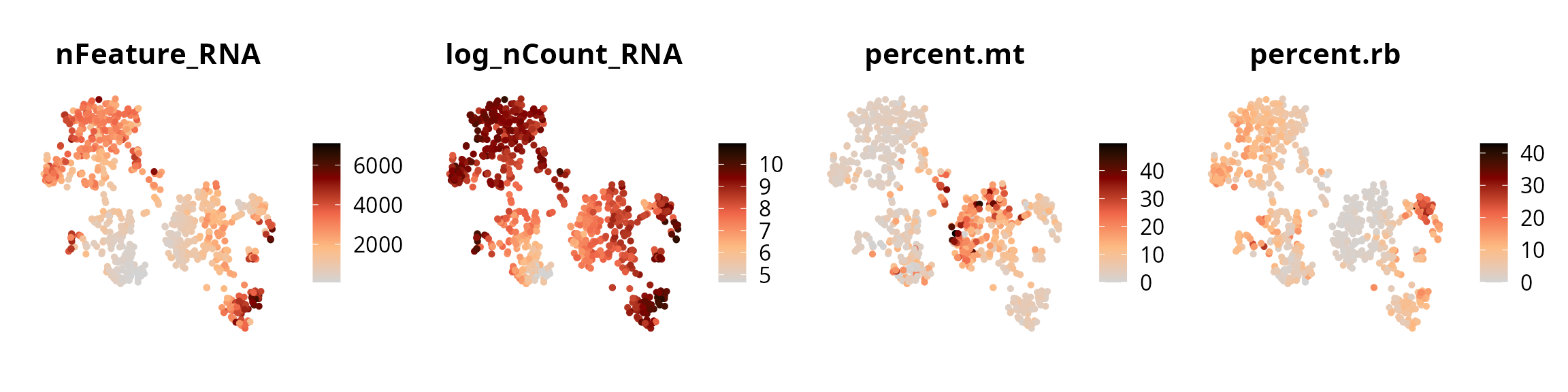
We make a Venn diagram of the failing cells to show the number of cells that fail the quality control because of more than one criterium.
n_filtered = c(fail_percent.mt, fail_percent.rb, fail_log_nCount_RNA, fail_nFeature_RNA) %>%
  unique() %>% length()
percent_filtered = round(100*(n_filtered/ncol(sobj)), 2)

ggvenn::ggvenn(list(percent.mt = fail_percent.mt,
                    percent.rb = fail_percent.rb,
                    log_nCount_RNA = fail_log_nCount_RNA,
                    nFeature_RNA = fail_nFeature_RNA),
               fill_color = c("#0073C2FF", "#EFC000FF", "orange", "pink"),
               stroke_size = 0.5, set_name_size = 4) +
  ggplot2::labs(title = "Filtered out cells",
                subtitle = paste0(n_filtered, " cells (", percent_filtered, " % of all cells)")) +
  ggplot2::theme(plot.title = element_text(hjust = 0.5, face = "bold"),
                 plot.subtitle = element_text(hjust = 0.5))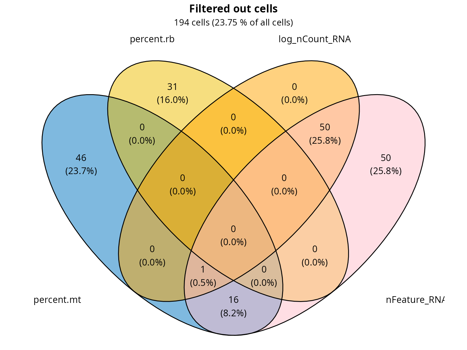
Knee plot
We make a knee plot, as on the web-summary from Cell Ranger:
data.frame(cell_bc = rownames(sobj@meta.data),
           nb_umi = sobj$nCount_RNA,
           nb_features = sobj$nFeature_RNA) %>%
  dplyr::arrange(-nb_umi) %>%
  dplyr::mutate(cell_rank = c(1:n())) %>%
  ggplot2::ggplot(., aes(x = cell_rank, y = nb_umi, col = nb_features)) +
  ggplot2::geom_point(size = 0.5) +
  ggplot2::labs(x = "Barcodes (Candidate cells)", y = "UMI counts") +
  ggplot2::geom_hline(yintercept = exp(cut_log_nCount_RNA), col = "red", lwd = 0.5) +
  ggplot2::scale_color_gradientn(colors = aquarius::palette_GrOrBl, name = "Feature counts") +
  ggplot2::scale_x_log10(breaks = scales::trans_breaks("log10", function(x) 10^x),
                         labels = scales::trans_format("log10", scales::math_format(10^.x)),
                         expand = expand_scale(mult = c(0, 0.05))) +
  ggplot2::scale_y_log10(breaks = scales::trans_breaks("log10", function(x) 10^x),
                         labels = scales::trans_format("log10", scales::math_format(10^.x)),
                         expand = expand_scale(mult = c(0.01, 0.05))) +
  ggplot2::theme_classic() +
  ggplot2::theme(panel.grid.major = element_line(color = "gray90"))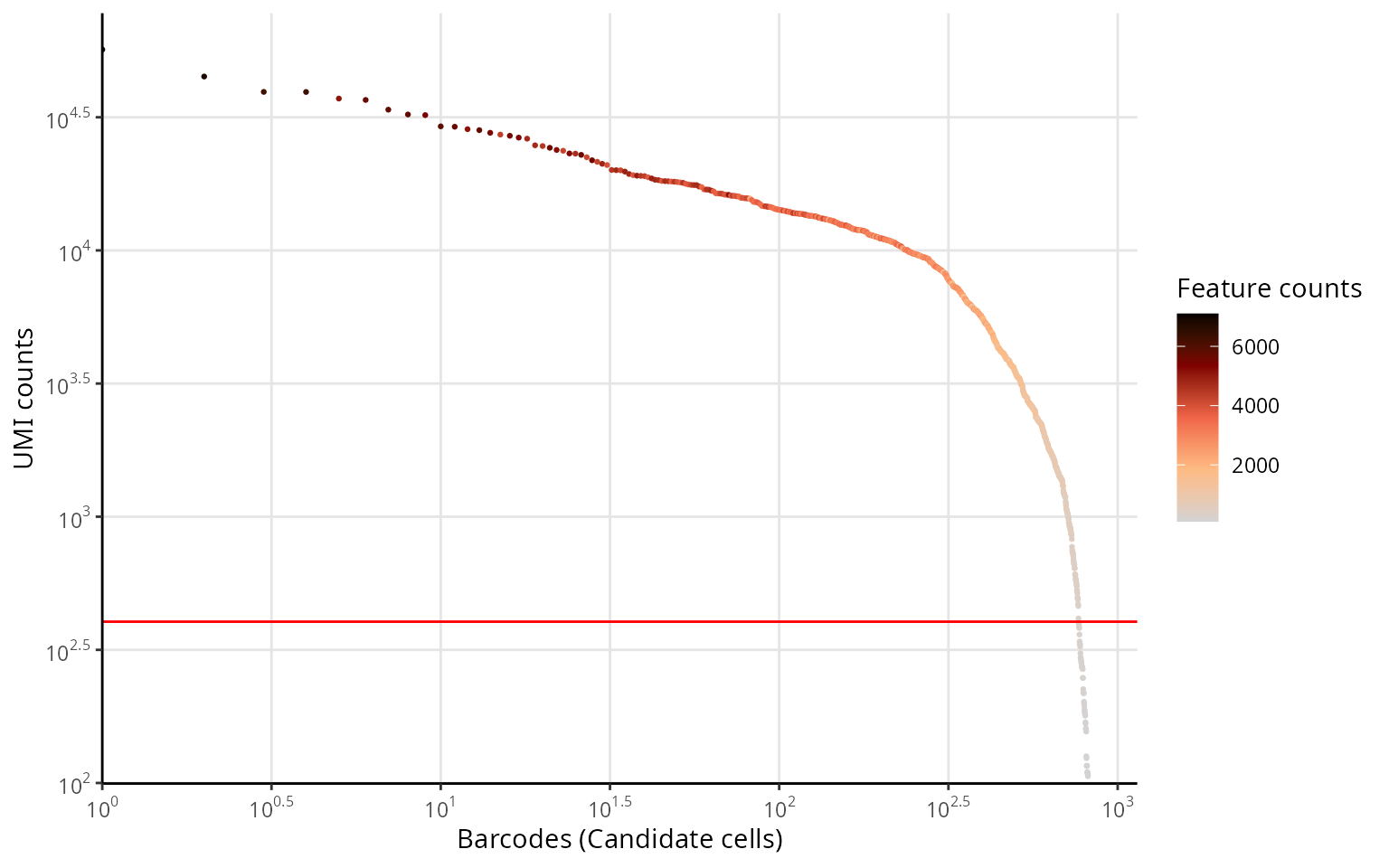
Number of UMI
To visualize the threshold for number of UMI, we can make a histogram:
aquarius::plot_qc_density(df = sobj@meta.data,
                          x = "log_nCount_RNA",
                          bins = 200,
                          group_by = "orig.ident",
                          group_color = sample_info[sample_name, "color"],
                          x_thresh = cut_log_nCount_RNA)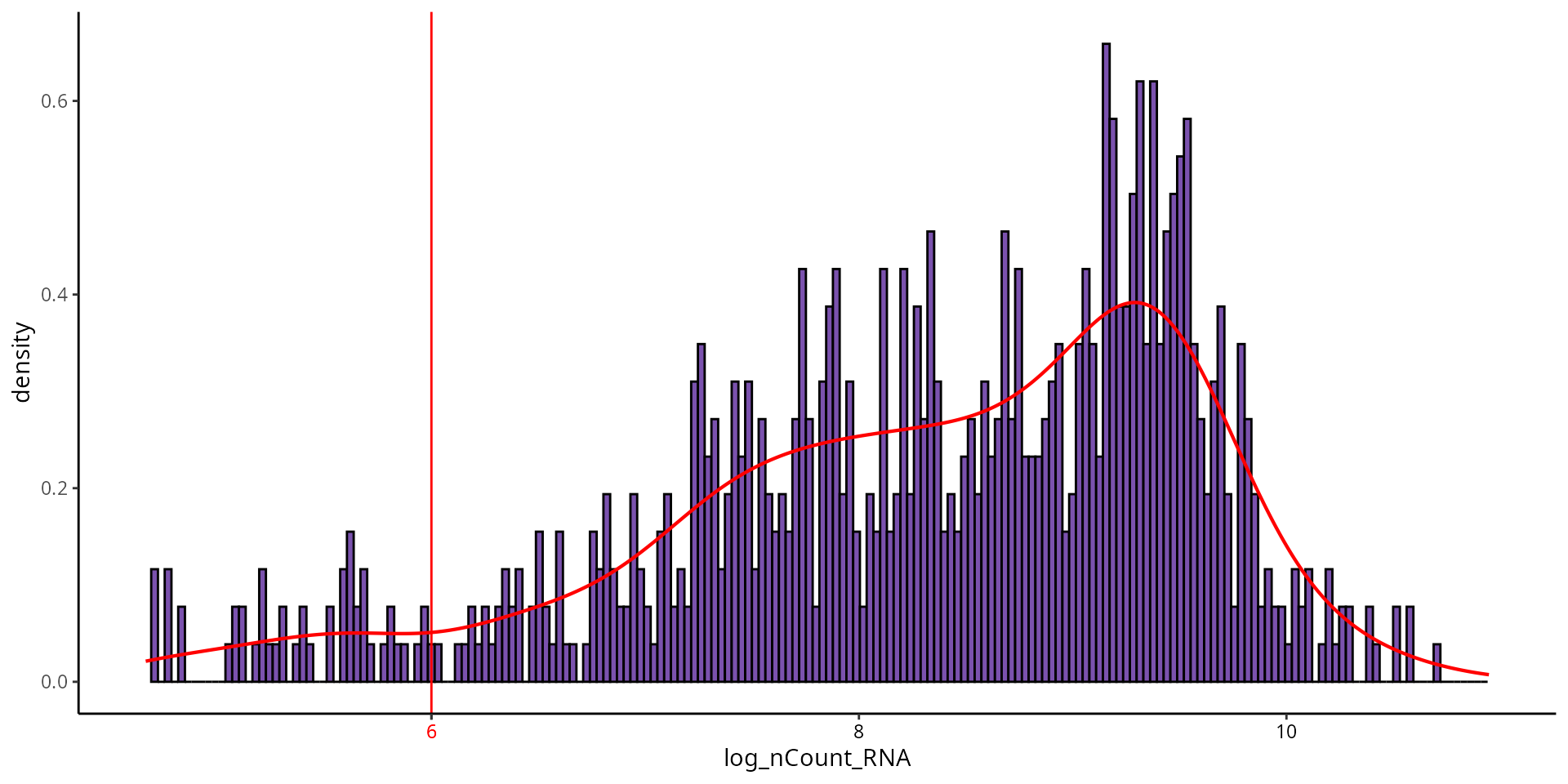
We visualize if there is a difference in the quality between annotated cell types.
Seurat::VlnPlot(sobj, features = "log_nCount_RNA", pt.size = 0.001,
                group.by = "cell_type", cols = color_markers) +
  ggplot2::scale_fill_manual(values = color_markers, breaks = names(color_markers)) +
  ggplot2::geom_hline(yintercept = cut_log_nCount_RNA, col = "red") +
  ggplot2::labs(x = "")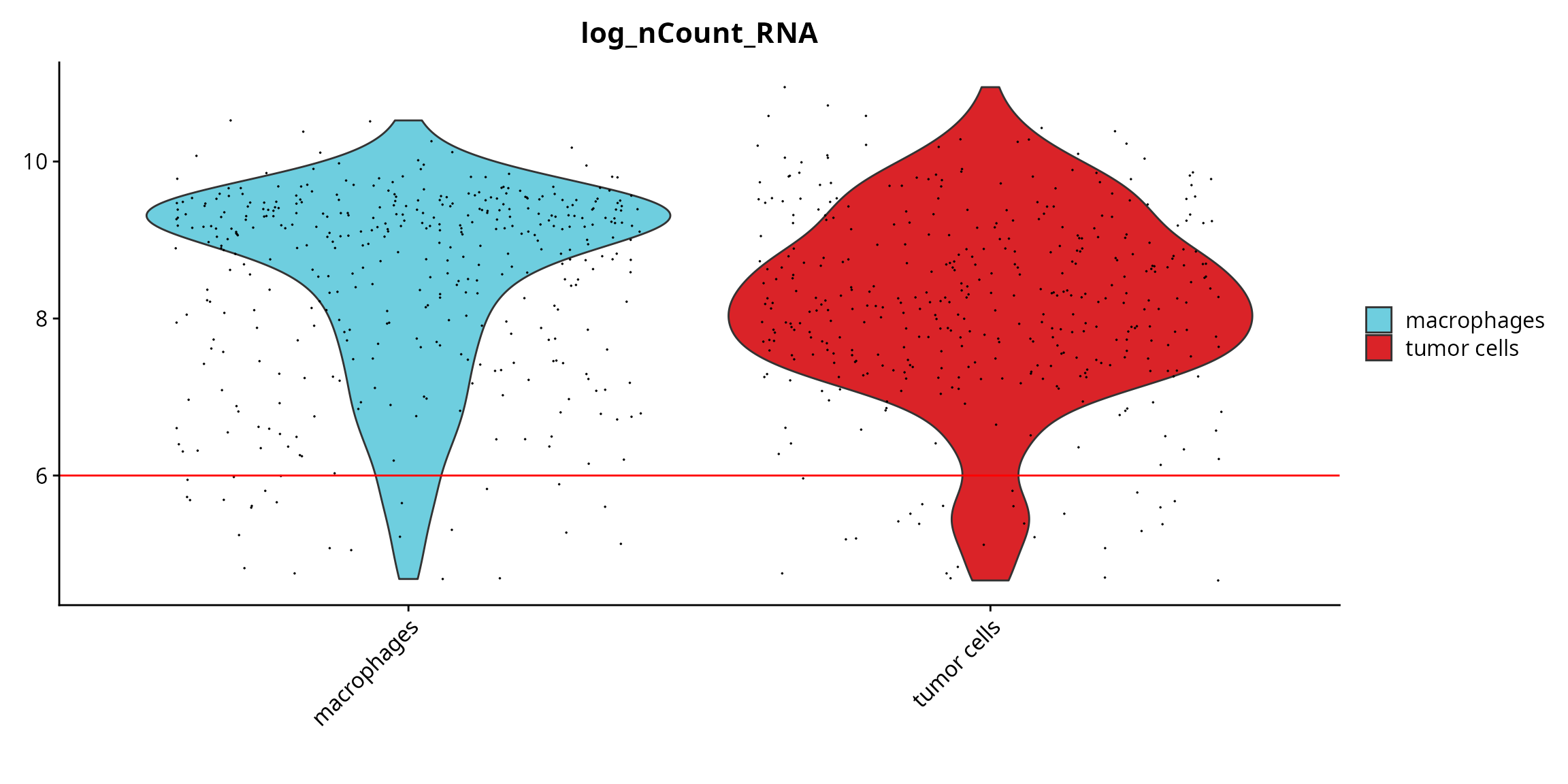
We visualize the failing cells on the projection, to check if they are grouped together (pool of low quality cells) or if they are spread over the projection (their profile, although of low quality, enables to separate cells).
sobj$fail = ifelse(colnames(sobj) %in% fail_log_nCount_RNA,
                   yes = as.character(sobj$cell_type), no = "kept cells")
sobj$fail = factor(sobj$fail, levels = c(levels(sobj$cell_type), "kept cells"))

p1 = Seurat::FeaturePlot(sobj, features = "log_nCount_RNA",
                         reduction = paste0("RNA_pca_", ndims, "_tsne")) +
  ggplot2::scale_color_gradientn(colors = aquarius::palette_GrOrBl) +
  Seurat::NoAxes() +
  ggplot2::theme(aspect.ratio = 1)

p2 = Seurat::DimPlot(sobj, group.by = "fail", reduction = paste0("RNA_pca_", ndims, "_tsne"),
                     cols = c(color_markers, list("kept cells" = "gray80"))) +
  ggplot2::labs(title = "log_nCount_RNA",
                subtitle = paste0(length(fail_log_nCount_RNA), " cells")) +
  Seurat::NoAxes() +
  ggplot2::theme(aspect.ratio = 1,
                 plot.title = element_text(hjust = 0.5),
                 plot.subtitle = element_text(hjust = 0.5))

p1 | p2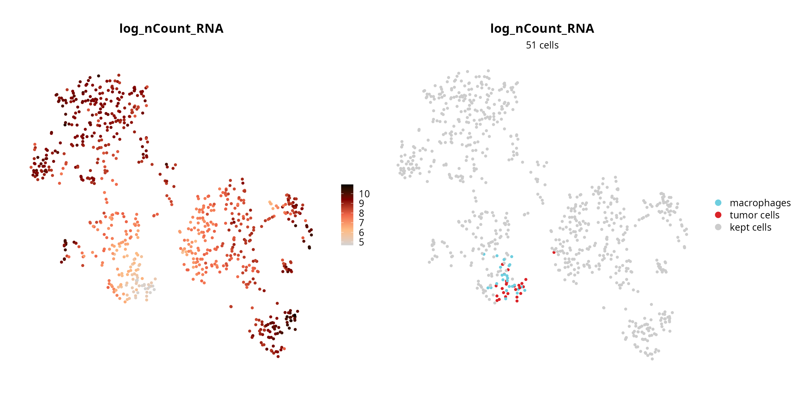
Number of features
To visualize the threshold for number of features, we can make a histogram:
aquarius::plot_qc_density(df = sobj@meta.data,
                          x = "nFeature_RNA",
                          bins = 200,
                          group_by = "orig.ident",
                          group_color = sample_info[sample_name, "color"],
                          x_thresh = cut_nFeature_RNA)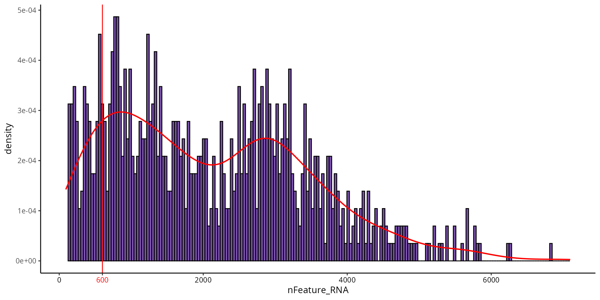
We visualize if there is a difference in the quality between annotated cell types.
Seurat::VlnPlot(sobj, features = "nFeature_RNA", pt.size = 0.001,
                group.by = "cell_type", cols = color_markers) +
  ggplot2::scale_fill_manual(values = color_markers, breaks = names(color_markers)) +
  ggplot2::geom_hline(yintercept = cut_nFeature_RNA, col = "red") +
  ggplot2::labs(x = "")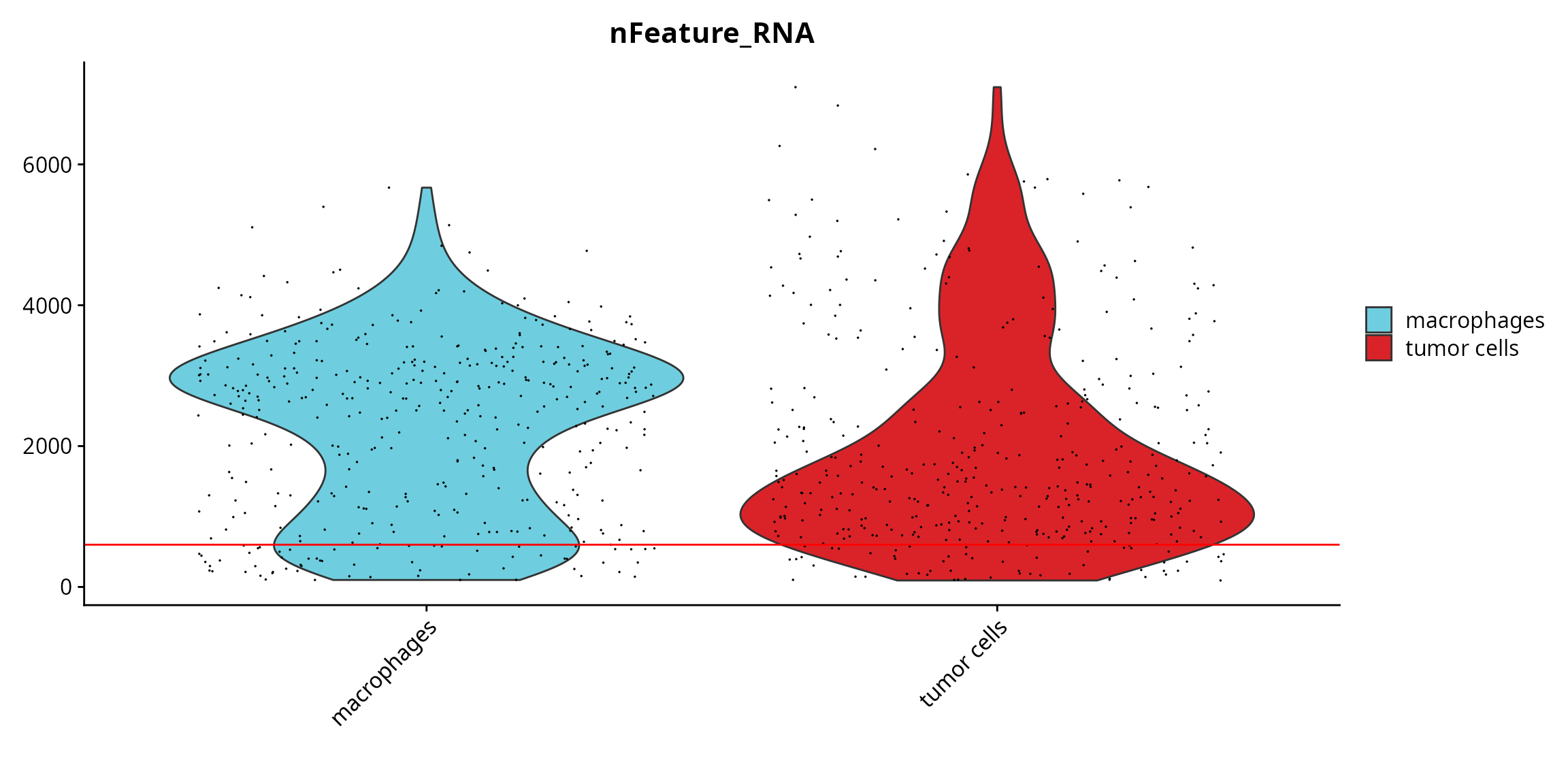
We visualize the failing cells on the projection, to check if they are grouped together (pool of low quality cells) or if they are spread over the projection (their profile, although of low quality, enables to separate cells).
sobj$fail = ifelse(colnames(sobj) %in% fail_nFeature_RNA,
                   yes = as.character(sobj$cell_type), no = "kept cells")
sobj$fail = factor(sobj$fail, levels = c(levels(sobj$cell_type), "kept cells"))

p1 = Seurat::FeaturePlot(sobj, features = "nFeature_RNA",
                         reduction = paste0("RNA_pca_", ndims, "_tsne")) +
  ggplot2::scale_color_gradientn(colors = aquarius::palette_GrOrBl) +
  Seurat::NoAxes() +
  ggplot2::theme(aspect.ratio = 1)

p2 = Seurat::DimPlot(sobj, group.by = "fail", reduction = paste0("RNA_pca_", ndims, "_tsne"),
                     cols = c(color_markers, list("kept cells" = "gray80"))) +
  ggplot2::labs(title = "nFeature_RNA",
                subtitle = paste0(length(fail_nFeature_RNA), " cells")) +
  Seurat::NoAxes() +
  ggplot2::theme(aspect.ratio = 1,
                 plot.title = element_text(hjust = 0.5),
                 plot.subtitle = element_text(hjust = 0.5))

p1 | p2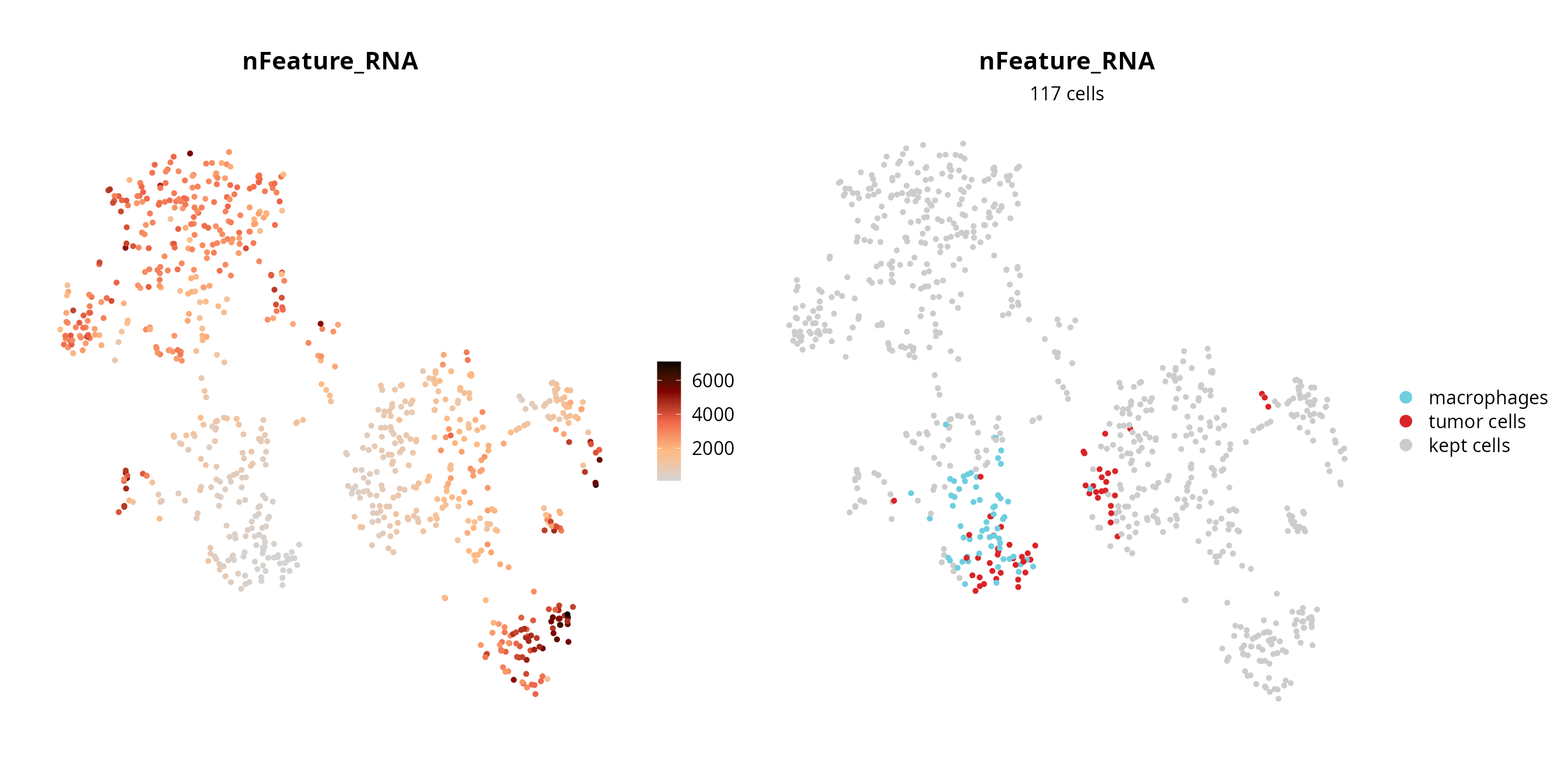
Mitochondrial genes expression
To identify a threshold for mitochondrial gene expression, we can make a histogram:
aquarius::plot_qc_density(df = sobj@meta.data,
                          x = "percent.mt",
                          bins = 200,
                          group_by = "orig.ident",
                          group_color = sample_info[sample_name, "color"],
                          x_thresh = cut_percent.mt)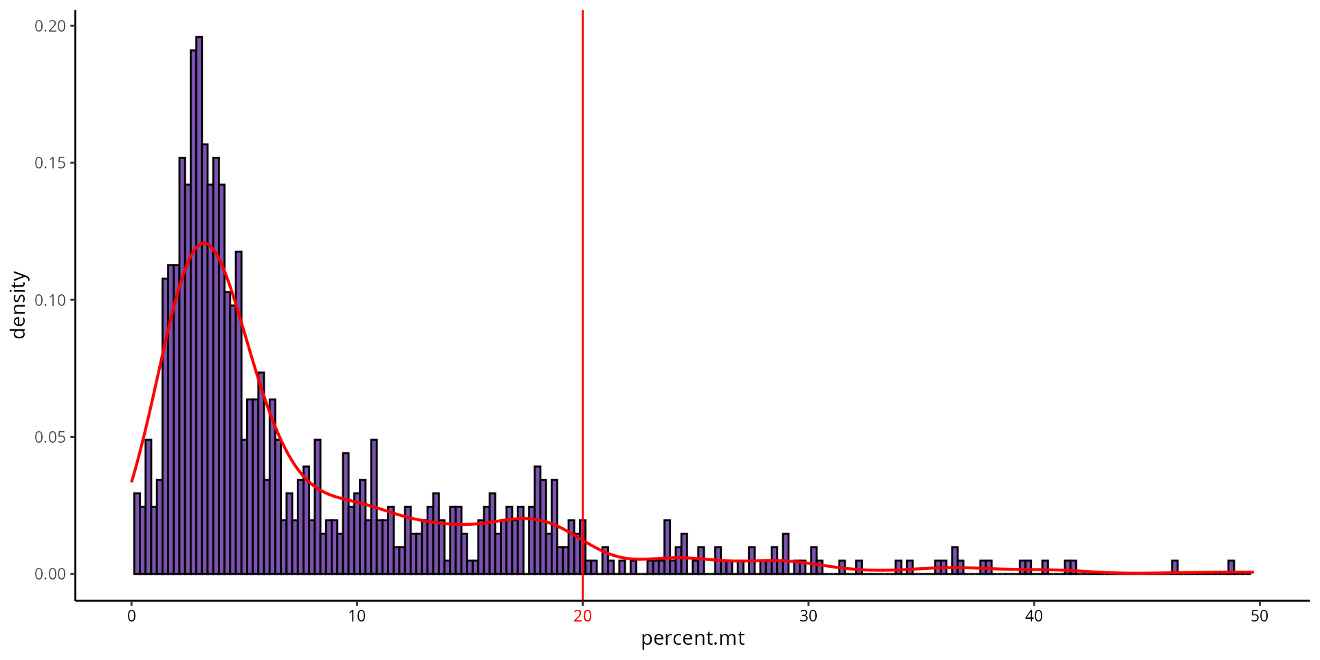
We visualize if there is a difference in the quality between annotated cell types.
Seurat::VlnPlot(sobj, features = "percent.mt", pt.size = 0.001,
                group.by = "cell_type", cols = color_markers) +
  ggplot2::scale_fill_manual(values = color_markers, breaks = names(color_markers)) +
  ggplot2::geom_hline(yintercept = cut_percent.mt, col = "red") +
  ggplot2::labs(x = "")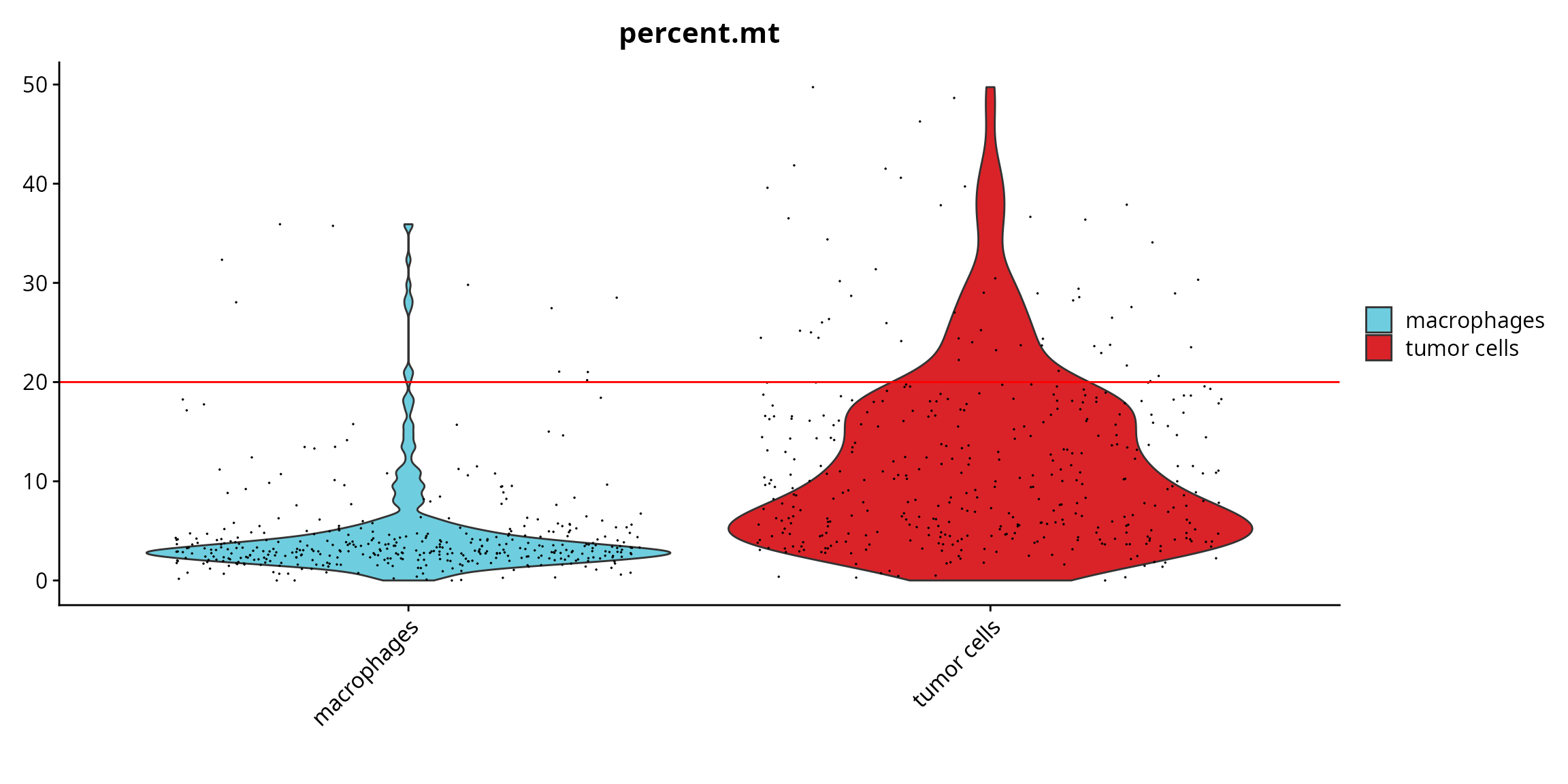
We visualize the failing cells on the projection, to check if they are grouped together (pool of low quality cells) or if they are spread over the projection (their profile, although of low quality, enables to separate cells).
sobj$fail = ifelse(colnames(sobj) %in% fail_percent.mt,
                   yes = as.character(sobj$cell_type), no = "kept cells")
sobj$fail = factor(sobj$fail, levels = c(levels(sobj$cell_type), "kept cells"))

p1 = Seurat::FeaturePlot(sobj, features = "percent.mt",
                         reduction = paste0("RNA_pca_", ndims, "_tsne")) +
  ggplot2::scale_color_gradientn(colors = aquarius::palette_GrOrBl) +
  Seurat::NoAxes() +
  ggplot2::theme(aspect.ratio = 1)

p2 = Seurat::DimPlot(sobj, group.by = "fail", reduction = paste0("RNA_pca_", ndims, "_tsne"),
                     cols = c(color_markers, list("kept cells" = "gray80"))) +
  ggplot2::labs(title = "percent.mt",
                subtitle = paste0(length(fail_percent.mt), " cells")) +
  Seurat::NoAxes() +
  ggplot2::theme(aspect.ratio = 1,
                 plot.title = element_text(hjust = 0.5),
                 plot.subtitle = element_text(hjust = 0.5))

p1 | p2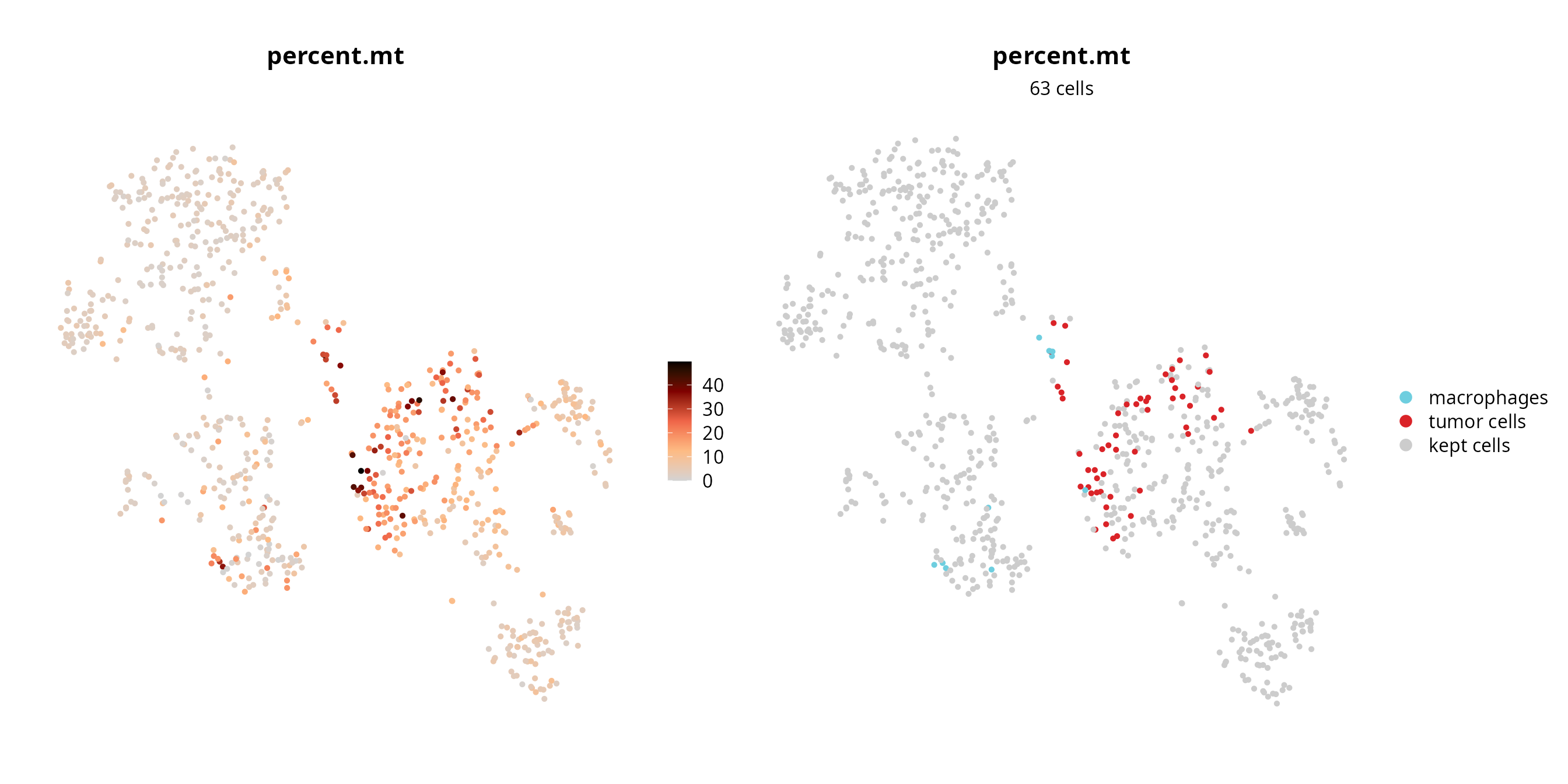
Ribosomal genes expression
To identify a threshold for ribosomal gene expression, we can make a histogram:
aquarius::plot_qc_density(df = sobj@meta.data,
                          x = "percent.rb",
                          bins = 200,
                          group_by = "orig.ident",
                          group_color = sample_info[sample_name, "color"],
                          x_thresh = cut_percent.rb)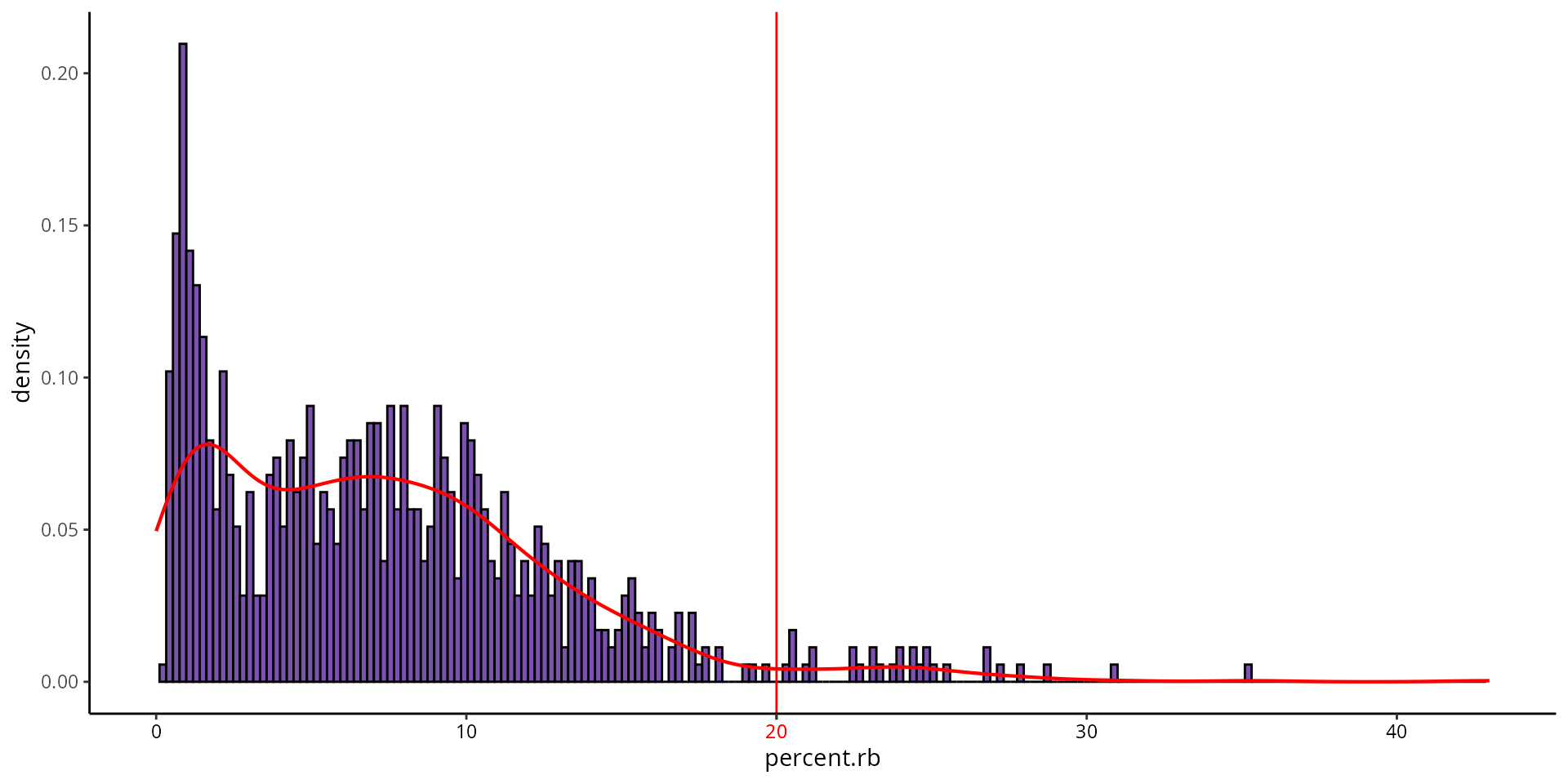
We visualize if there is a difference in the quality between annotated cell types.
Seurat::VlnPlot(sobj, features = "percent.rb", pt.size = 0.001,
                group.by = "cell_type", cols = color_markers) +
  ggplot2::scale_fill_manual(values = color_markers, breaks = names(color_markers)) +
  ggplot2::geom_hline(yintercept = cut_percent.rb, col = "red") +
  ggplot2::labs(x = "")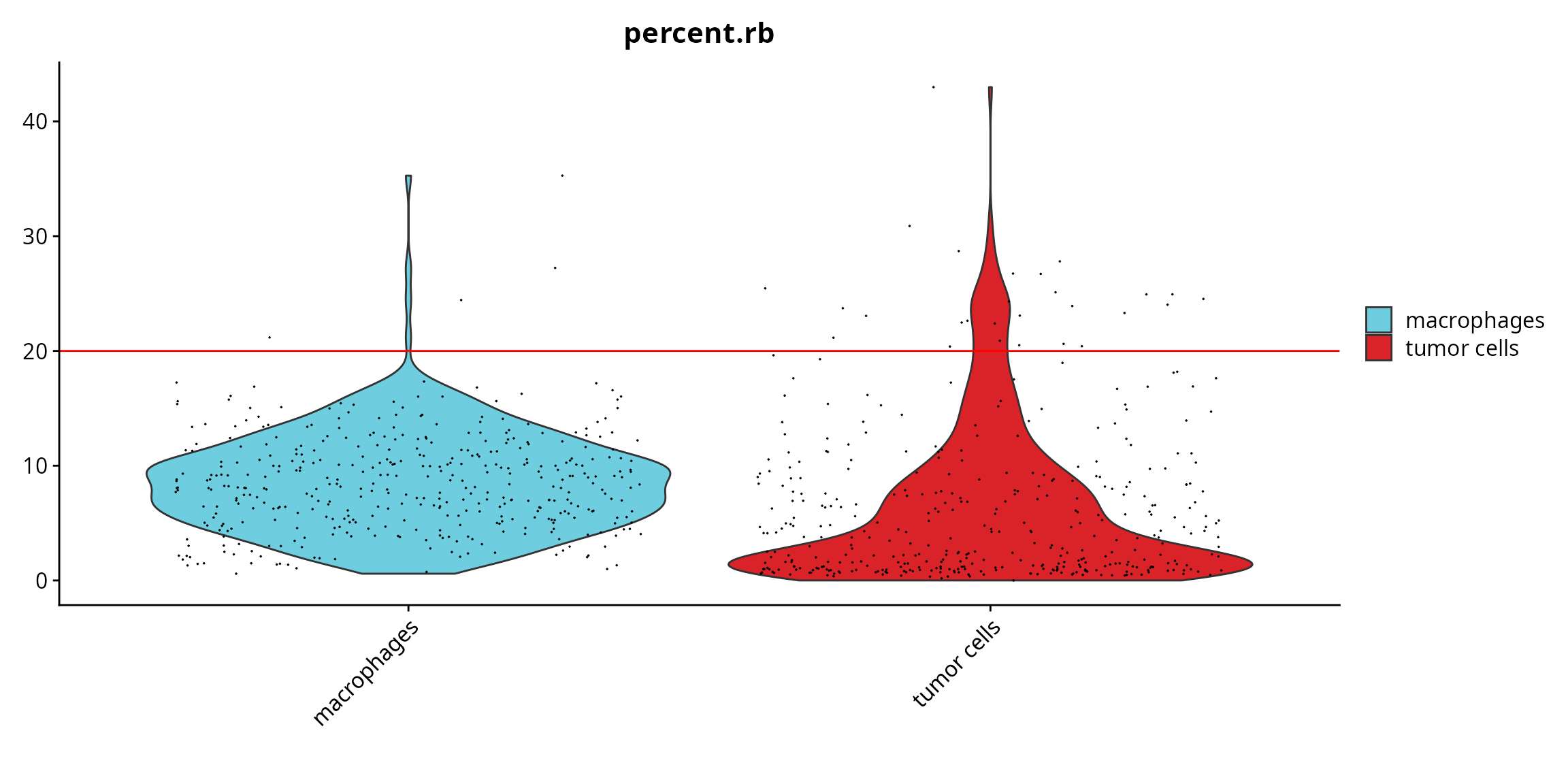
We visualize the failing cells on the projection, to check if they are grouped together (pool of low quality cells) or if they are spread over the projection (their profile, although of low quality, enables to separate cells).
sobj$fail = ifelse(colnames(sobj) %in% fail_percent.rb,
                   yes = as.character(sobj$cell_type), no = "kept cells")
sobj$fail = factor(sobj$fail, levels = c(levels(sobj$cell_type), "kept cells"))

p1 = Seurat::FeaturePlot(sobj, features = "percent.rb",
                         reduction = paste0("RNA_pca_", ndims, "_tsne")) +
  ggplot2::scale_color_gradientn(colors = aquarius::palette_GrOrBl) +
  Seurat::NoAxes() +
  ggplot2::theme(aspect.ratio = 1)

p2 = Seurat::DimPlot(sobj, group.by = "fail", reduction = paste0("RNA_pca_", ndims, "_tsne"),
                     cols = c(color_markers, list("kept cells" = "gray80"))) +
  ggplot2::labs(title = "percent.rb",
                subtitle = paste0(length(fail_percent.rb), " cells")) +
  Seurat::NoAxes() +
  ggplot2::theme(aspect.ratio = 1,
                 plot.title = element_text(hjust = 0.5),
                 plot.subtitle = element_text(hjust = 0.5))

p1 | p2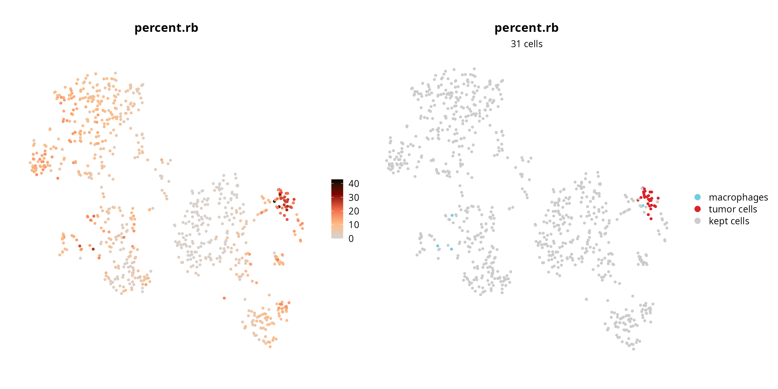
FACS-like figure
We would like to see if the number of feature expressed by cell, and
the number of UMI is correlated with the cell type, the percentage of
mitochondrial and ribosomal gene expressed, and the doublet status. We
build the log_nCount_RNA by nFeature_RNA
figure, where cells (dots) are colored by these different metrics. This
is just another way to apprehend the quality control.
This is the figure, colored by cell type:
aquarius::plot_qc_facslike(df = sobj@meta.data,
                           x = "nFeature_RNA",
                           y = "log_nCount_RNA",
                           col_by = "cell_type",
                           col_colors = unname(color_markers),
                           x_thresh = cut_nFeature_RNA,
                           y_thresh = cut_log_nCount_RNA,
                           bins = 200)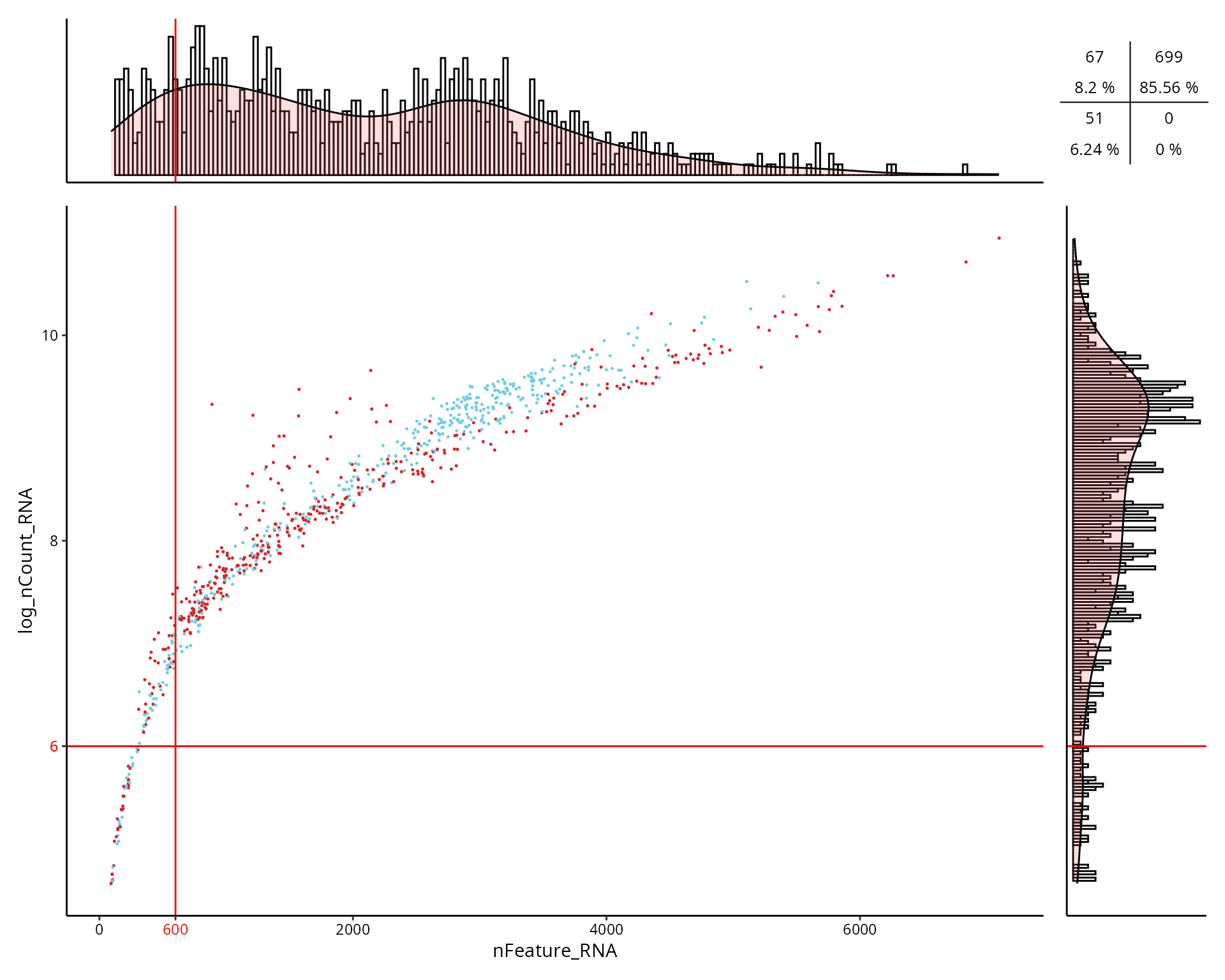
This is the figure, colored by the percentage of mitochondrial genes expressed in cell:
aquarius::plot_qc_facslike(df = sobj@meta.data,
                           x = "nFeature_RNA",
                           y = "log_nCount_RNA",
                           col_by = "percent.mt",
                           x_thresh = cut_nFeature_RNA,
                           y_thresh = cut_log_nCount_RNA,
                           bins = 200)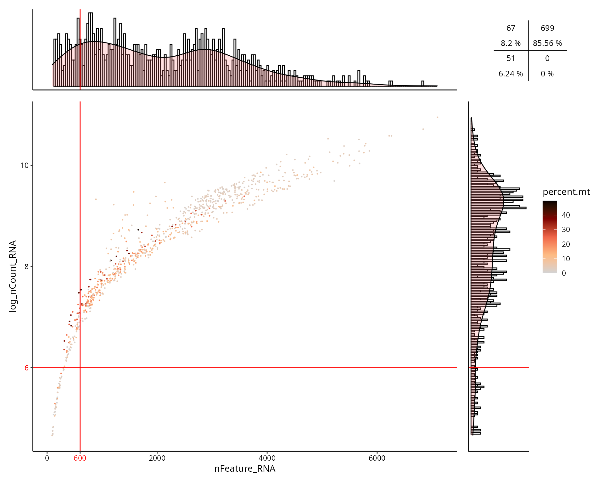
This is the figure, colored by the percentage of ribosomal genes expressed in cell:
aquarius::plot_qc_facslike(df = sobj@meta.data,
                           x = "nFeature_RNA",
                           y = "log_nCount_RNA",
                           col_by = "percent.rb",
                           x_thresh = cut_nFeature_RNA,
                           y_thresh = cut_log_nCount_RNA,
                           bins = 200)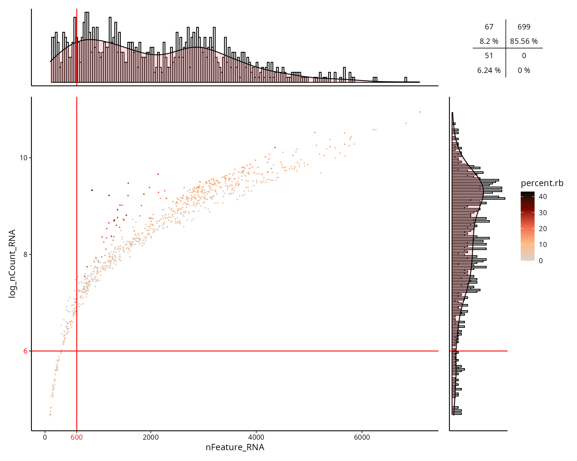
This is the figure, colored by the doublet cells status
(doublets_consensus.class):
aquarius::plot_qc_facslike(df = sobj@meta.data,
                           x = "nFeature_RNA",
                           y = "log_nCount_RNA",
                           col_by = "doublets_consensus.class",
                           col_colors = setNames(nm = c(TRUE, FALSE),
                                                 aquarius::gg_color_hue(2)),
                           x_thresh = cut_nFeature_RNA,
                           y_thresh = cut_log_nCount_RNA,
                           bins = 200)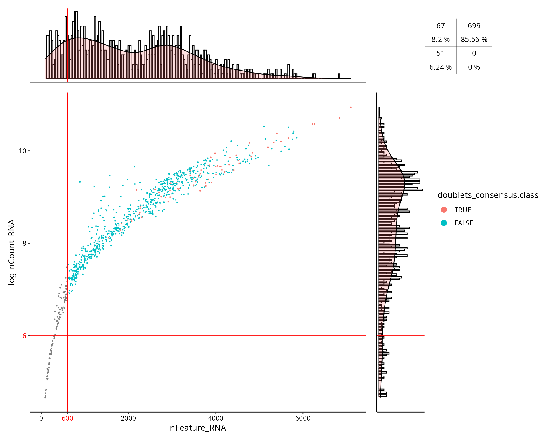
This is the figure, colored by the doublet cells status
(scDblFinder.class):
aquarius::plot_qc_facslike(df = sobj@meta.data,
                           x = "nFeature_RNA",
                           y = "log_nCount_RNA",
                           col_by = "scDblFinder.class",
                           col_colors = setNames(nm = c(TRUE, FALSE),
                                                 aquarius::gg_color_hue(2)),
                           x_thresh = cut_nFeature_RNA,
                           y_thresh = cut_log_nCount_RNA,
                           bins = 200)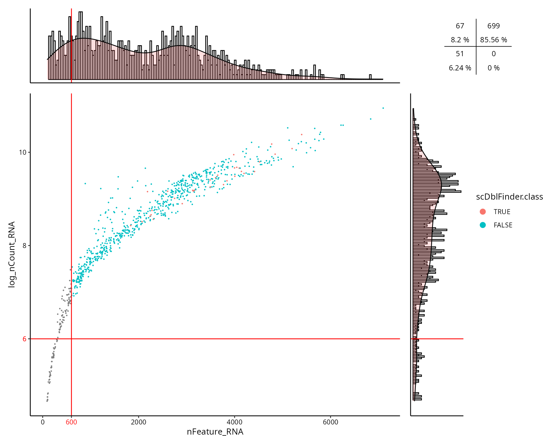
This is the figure, colored by the doublet cells status
(hybrid_score.class):
aquarius::plot_qc_facslike(df = sobj@meta.data,
                           x = "nFeature_RNA",
                           y = "log_nCount_RNA",
                           col_by = "hybrid_score.class",
                           col_colors = setNames(nm = c(TRUE, FALSE),
                                                 aquarius::gg_color_hue(2)),
                           x_thresh = cut_nFeature_RNA,
                           y_thresh = cut_log_nCount_RNA,
                           bins = 200)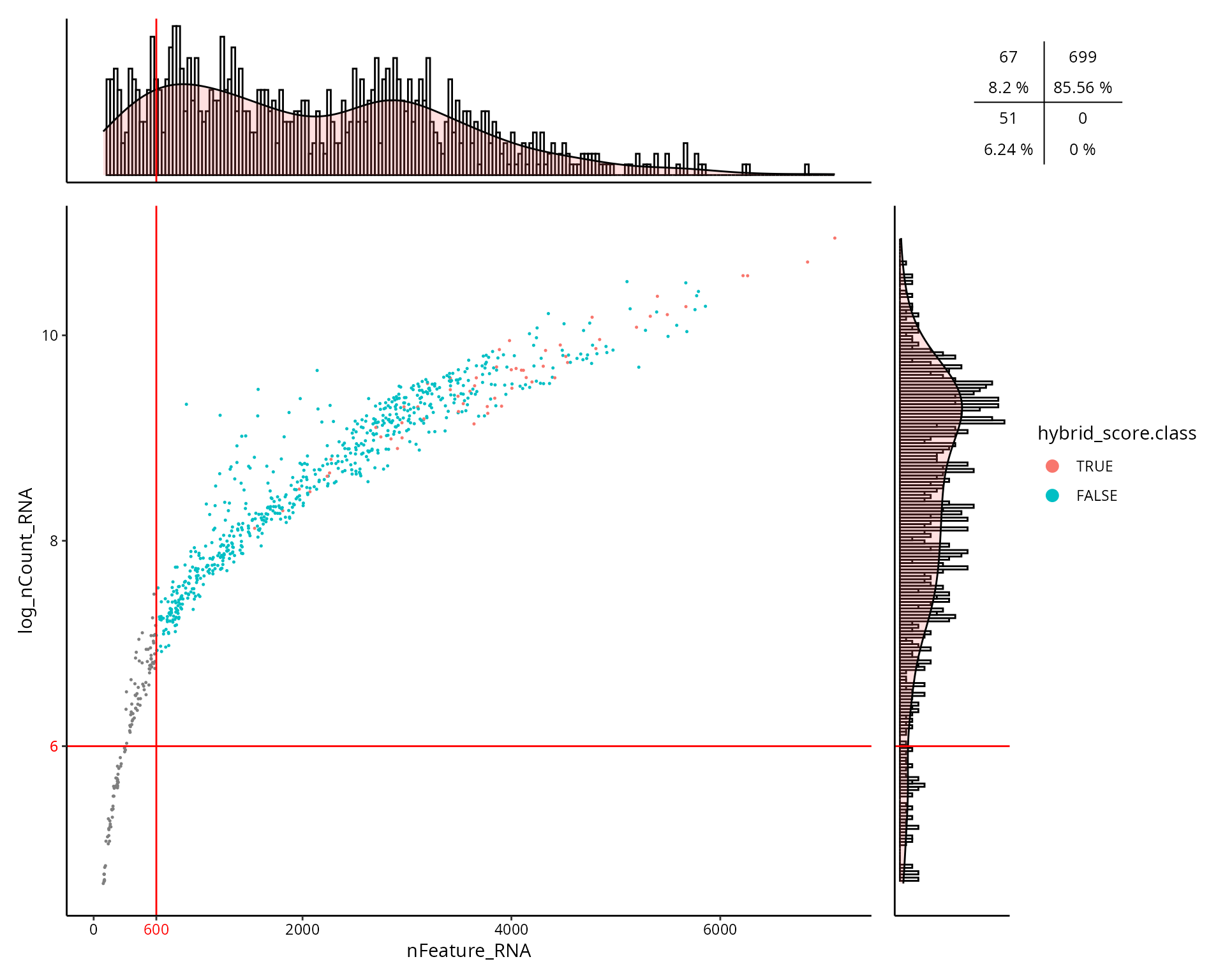
Visualization as piechart
Do filtered cells belong to a particular cell type ?
sobj$all_cells = TRUE

piechart_all_cells = aquarius::plot_piechart(df = sobj@meta.data,
                                             logical_var = "all_cells",
                                             grouping_var = "cell_type",
                                             colors = color_markers,
                                             display_legend = TRUE) +
  ggplot2::labs(title = "All cells",
                subtitle = paste(nrow(sobj@meta.data), "cells")) +
  ggplot2::theme(plot.title = element_text(hjust = 0.5, face = "bold"),
                 plot.subtitle = element_text(hjust = 0.5))

piechart_doublets = aquarius::plot_piechart(df = sobj@meta.data %>%
                                              dplyr::filter(doublets_consensus.class),
                                            logical_var = "all_cells",
                                            grouping_var = "cell_type",
                                            colors = color_markers,
                                            display_legend = TRUE) +
  ggplot2::labs(title = "doublets_consensus.class",
                subtitle = paste(sum(sobj$doublets_consensus.class, na.rm = TRUE), "cells")) +
  ggplot2::theme(plot.title = element_text(hjust = 0.5, face = "bold"),
                 plot.subtitle = element_text(hjust = 0.5))

piechart_percent.mt = aquarius::plot_piechart(df = sobj@meta.data %>%
                                                dplyr::filter(percent.mt > cut_percent.mt),
                                              logical_var = "all_cells",
                                              grouping_var = "cell_type",
                                              colors = color_markers,
                                              display_legend = TRUE) +
  ggplot2::labs(title = paste("percent.mt >", cut_percent.mt),
                subtitle = paste(length(fail_percent.mt), "cells")) +
  ggplot2::theme(plot.title = element_text(hjust = 0.5, face = "bold"),
                 plot.subtitle = element_text(hjust = 0.5))

piechart_percent.rb = aquarius::plot_piechart(df = sobj@meta.data %>%
                                                dplyr::filter(percent.rb > cut_percent.rb),
                                              logical_var = "all_cells",
                                              grouping_var = "cell_type",
                                              colors = color_markers,
                                              display_legend = TRUE) +
  ggplot2::labs(title = paste("percent.rb >", cut_percent.rb),
                subtitle = paste(length(fail_percent.rb), "cells")) +
  ggplot2::theme(plot.title = element_text(hjust = 0.5, face = "bold"),
                 plot.subtitle = element_text(hjust = 0.5))

piechart_log_nCount_RNA = aquarius::plot_piechart(df = sobj@meta.data %>%
                                                    dplyr::filter(log_nCount_RNA < cut_log_nCount_RNA),
                                                  logical_var = "all_cells",
                                                  grouping_var = "cell_type",
                                                  colors = color_markers,
                                                  display_legend = TRUE) +
  ggplot2::labs(title = paste("log_nCount_RNA <", round(cut_log_nCount_RNA, 2)),
                subtitle = paste(length(fail_log_nCount_RNA), "cells")) +
  ggplot2::theme(plot.title = element_text(hjust = 0.5, face = "bold"),
                 plot.subtitle = element_text(hjust = 0.5))

piechart_nFeature_RNA = aquarius::plot_piechart(df = sobj@meta.data %>%
                                                  dplyr::filter(nFeature_RNA < cut_nFeature_RNA),
                                                logical_var = "all_cells",
                                                grouping_var = "cell_type",
                                                colors = color_markers,
                                                display_legend = TRUE) +
  ggplot2::labs(title = paste("nFeature_RNA <", round(cut_nFeature_RNA, 2)),
                subtitle = paste(length(fail_nFeature_RNA), "cells")) +
  ggplot2::theme(plot.title = element_text(hjust = 0.5, face = "bold"),
                 plot.subtitle = element_text(hjust = 0.5))

patchwork::wrap_plots(piechart_all_cells, piechart_percent.mt, piechart_percent.rb,
                      piechart_doublets, piechart_nFeature_RNA, piechart_log_nCount_RNA) +
  patchwork::plot_layout(guides = "collect") &
  ggplot2::theme(legend.position = "right")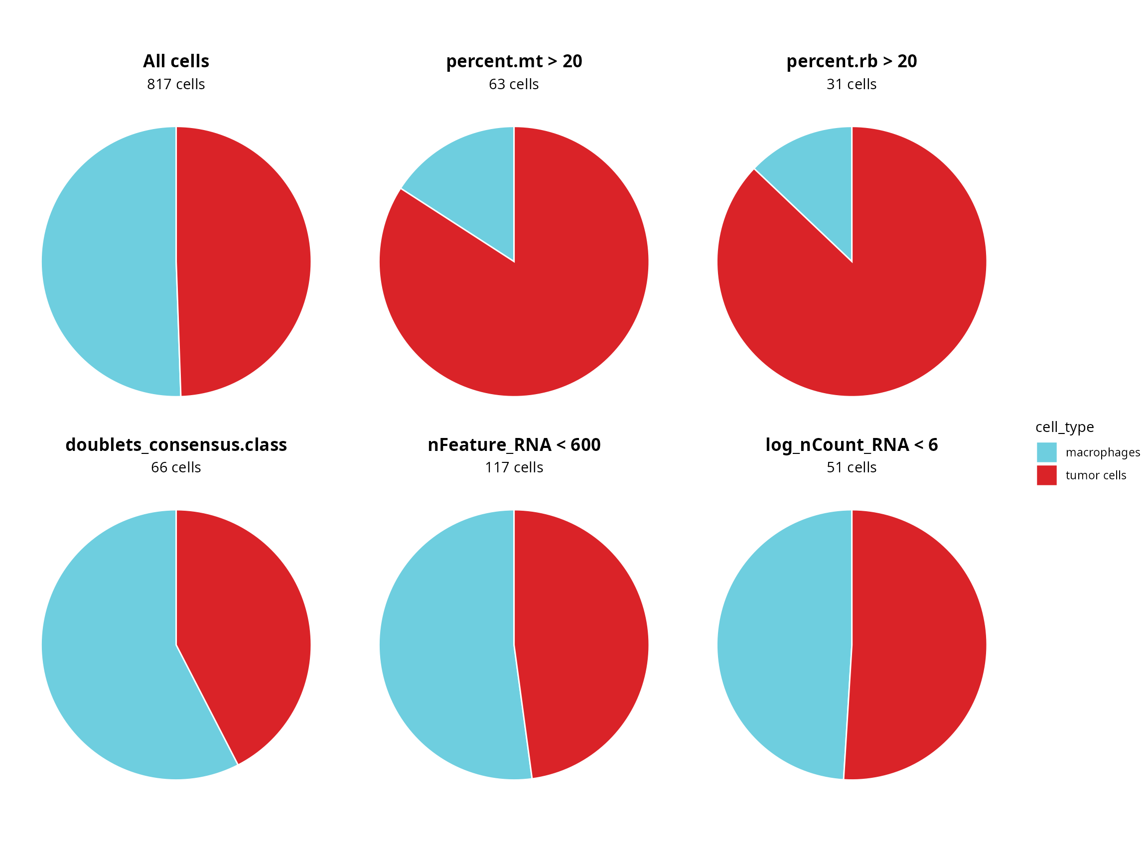
Doublet cells status
We can compare doublet detection methods with a Venn diagram:
ggvenn::ggvenn(list(hybrid = fail_doublets_hybrid,
                    scDblFinder = fail_doublets_scDblFinder),
               fill_color = c("#0073C2FF", "#EFC000FF"),
               stroke_size = 0.5, set_name_size = 4) +
  ggplot2::ggtitle(label = "Doublet cells") +
  ggplot2::theme(plot.title = element_text(hjust = 0.5, face = "bold"))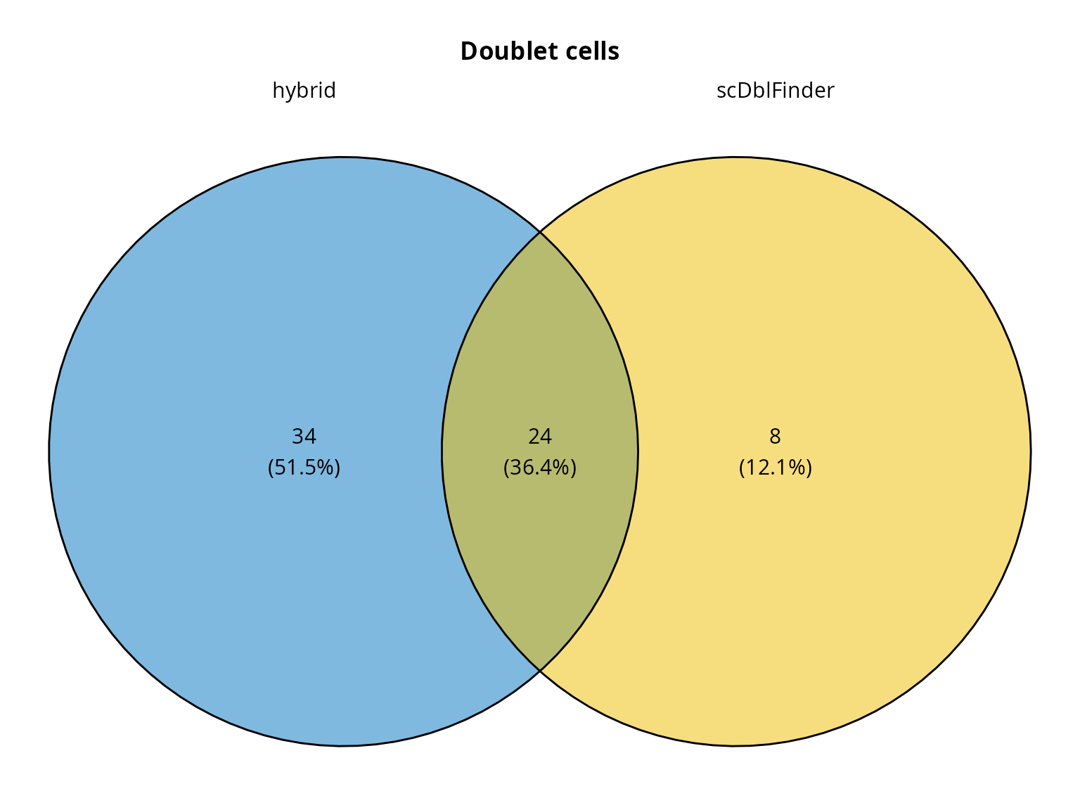
We visualize cells annotation for doublets. It can inform about their composition, because heterotypic doublet cells suffer from annotation competition between the two cell types they are annotated with.
plot_list = list()

# scDblFinder.class
sobj$fail = ifelse(sobj$scDblFinder.class,
                   yes = as.character(sobj$cell_type), no = "kept cells")
sobj$fail = factor(sobj$fail, levels = c(levels(sobj$cell_type), "kept cells"))

plot_list[[1]] = Seurat::DimPlot(sobj, group.by = "fail", reduction = paste0("RNA_pca_", ndims, "_tsne"),
                                 cols = c(color_markers, list("kept cells" = "gray80"))) +
  ggplot2::labs(title = "scDblFinder.class",
                subtitle = paste0(sum(sobj$scDblFinder.class, na.rm = TRUE), " cells")) +
  Seurat::NoAxes() + Seurat::NoLegend() +
  ggplot2::theme(aspect.ratio = 1,
                 plot.title = element_text(hjust = 0.5),
                 plot.subtitle = element_text(hjust = 0.5))

# hybrid_score.class
sobj$fail = ifelse(sobj$hybrid_score.class,
                   yes = as.character(sobj$cell_type), no = "kept cells")
sobj$fail = factor(sobj$fail, levels = c(levels(sobj$cell_type), "kept cells"))

plot_list[[2]] = Seurat::DimPlot(sobj, group.by = "fail", reduction = paste0("RNA_pca_", ndims, "_tsne"),
                                 cols = c(color_markers, list("kept cells" = "gray80"))) +
  ggplot2::labs(title = "hybrid_score.class",
                subtitle = paste0(sum(sobj$hybrid_score.class, na.rm = TRUE), " cells")) +
  Seurat::NoAxes() +
  ggplot2::theme(aspect.ratio = 1,
                 plot.title = element_text(hjust = 0.5),
                 plot.subtitle = element_text(hjust = 0.5))

sobj$fail = NULL

# Plot
patchwork::wrap_plots(plot_list, nrow = 1)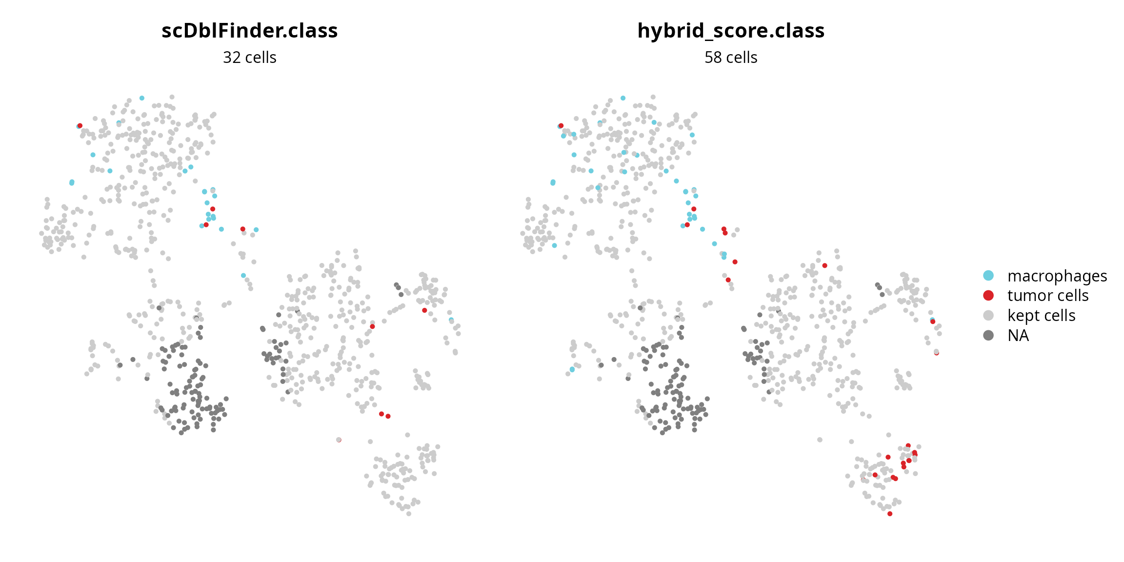
What is the composition of doublet cells ? We just look at scores for each cell type.
score_columns = grep(x = colnames(sobj@meta.data),
                     pattern = "^score",
                     value = TRUE)
combinations = expand.grid(score_columns, score_columns) %>%
  apply(., 1, sort) %>% t() %>%
  as.data.frame()
combinations = combinations[!duplicated(combinations), ]
combinations
## V1 V2
## 1 score_macrophages score_macrophages
## 2 score_macrophages score_tumor_cells
## 4 score_tumor_cells score_tumor_cellsWe prepare each figure:
plot_list = apply(combinations, 1, FUN = function(elem) {
  aquarius::plot_doublets_composition(sobj,
                                      score1 = elem[1],
                                      score2 = elem[2],
                                      doublet_annotation = "doublets_consensus.class")
})

sobj$orig.ident.doublets = NULL

patchwork::wrap_plots(plot_list) +
  patchwork::plot_layout(guides = "collect") &
  ggplot2::theme(legend.position = "right")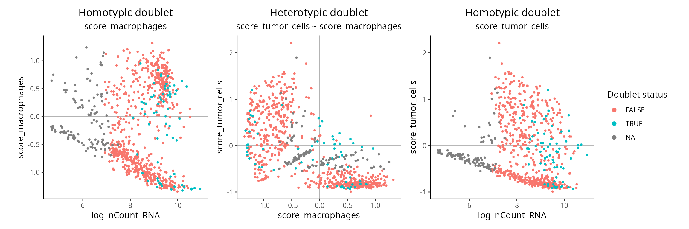
Filtering annotation
To further filter the object based on the quality metrics, we add the filtering information in the object.
sobj$fail_qc = ifelse(colnames(sobj) %in% c(fail_log_nCount_RNA, fail_nFeature_RNA,
                                            fail_percent.mt, fail_percent.rb,
                                            fail_doublets_consensus),
                      yes = TRUE, no = FALSE)

table(sobj$fail_qc)
##
## FALSE TRUE
## 563 254What is the content of metadata ?
summary(sobj@meta.data)## orig.ident nCount_RNA nFeature_RNA log_nCount_RNA score_macrophages
## A:817 Min. : 106 Min. : 92 Min. : 4.663 Min. :-1.3456
## 1st Qu.: 1965 1st Qu.: 924 1st Qu.: 7.583 1st Qu.:-0.8058
## Median : 5299 Median :1924 Median : 8.575 Median :-0.2087
## Mean : 7229 Mean :2105 Mean : 8.333 Mean :-0.1525
## 3rd Qu.:11002 3rd Qu.:3066 3rd Qu.: 9.306 3rd Qu.: 0.5406
## Max. :56790 Max. :7097 Max. :10.947 Max. : 1.3188
##
## score_tumor_cells cell_type Seurat.Phase cyclone.Phase
## Min. :-0.9899 macrophages:413 Length:817 Length:817
## 1st Qu.:-0.7875 tumor cells:404 Class :character Class :character
## Median :-0.3143 Mode :character Mode :character
## Mean :-0.1463
## 3rd Qu.: 0.3578
## Max. : 2.2130
##
## RNA_snn_res.0.5 seurat_clusters percent.mt percent.rb
## 0 :232 0 :232 Min. : 0.000 Min. : 0.000
## 1 :226 1 :226 1st Qu.: 2.866 1st Qu.: 2.475
## 2 :145 2 :145 Median : 4.624 Median : 6.631
## 3 : 82 3 : 82 Mean : 8.151 Mean : 7.383
## 4 : 52 4 : 52 3rd Qu.:10.995 3rd Qu.:10.369
## 5 : 50 5 : 50 Max. :49.735 Max. :42.983
## (Other): 30 (Other): 30
## doublets_consensus.class scDblFinder.class hybrid_score.class fail_qc
## Mode :logical Mode :logical Mode :logical Mode :logical
## FALSE:634 FALSE:668 FALSE:642 FALSE:563
## TRUE :66 TRUE :32 TRUE :58 TRUE :254
## NA's :117 NA's :117 NA's :117
##
##
## R Session
show
## R version 4.4.3 (2025-02-28)
## Platform: x86_64-pc-linux-gnu
## Running under: Ubuntu 24.10
##
## Matrix products: default
## BLAS:   /usr/lib/x86_64-linux-gnu/blas/libblas.so.3.12.0
## LAPACK: /usr/lib/x86_64-linux-gnu/lapack/liblapack.so.3.12.0
##
## locale:
##  [1] LC_CTYPE=en_US.UTF-8       LC_NUMERIC=C
##  [3] LC_TIME=fr_FR.UTF-8        LC_COLLATE=en_US.UTF-8
##  [5] LC_MONETARY=fr_FR.UTF-8    LC_MESSAGES=en_US.UTF-8
##  [7] LC_PAPER=fr_FR.UTF-8       LC_NAME=C
##  [9] LC_ADDRESS=C               LC_TELEPHONE=C
## [11] LC_MEASUREMENT=fr_FR.UTF-8 LC_IDENTIFICATION=C
##
## time zone: Europe/Paris
## tzcode source: system (glibc)
##
## attached base packages:
## [1] stats     graphics  grDevices utils     datasets  methods   base
##
## other attached packages:
## [1] future_1.40.0   ggplot2_3.5.2   patchwork_1.3.0 dplyr_1.1.4
##
## loaded via a namespace (and not attached):
##   [1] fs_1.6.6                    matrixStats_1.5.0
##   [3] spatstat.sparse_3.1-0       bitops_1.0-9
##   [5] httr_1.4.7                  RColorBrewer_1.1-3
##   [7] doParallel_1.0.17           tools_4.4.3
##   [9] sctransform_0.4.2           R6_2.6.1
##  [11] HDF5Array_1.34.0            lazyeval_0.2.2
##  [13] uwot_0.2.3                  rhdf5filters_1.18.1
##  [15] GetoptLong_1.0.5            withr_3.0.2
##  [17] sp_2.2-0                    gridExtra_2.3
##  [19] progressr_0.15.1            cli_3.6.5
##  [21] Biobase_2.66.0              textshaping_1.0.1
##  [23] aquarius_1.0.0              spatstat.explore_3.4-2
##  [25] fastDummies_1.7.5           labeling_0.4.3
##  [27] sass_0.4.10                 Seurat_5.3.0
##  [29] spatstat.data_3.1-6         ggridges_0.5.6
##  [31] pbapply_1.7-2               pkgdown_2.1.2
##  [33] Rsamtools_2.22.0            systemfonts_1.2.3
##  [35] R.utils_2.13.0              scater_1.34.1
##  [37] parallelly_1.43.0           limma_3.62.2
##  [39] generics_0.1.3              shape_1.4.6.1
##  [41] BiocIO_1.16.0               ica_1.0-3
##  [43] spatstat.random_3.3-3       Matrix_1.7-3
##  [45] ggbeeswarm_0.7.2            S4Vectors_0.44.0
##  [47] abind_1.4-8                 R.methodsS3_1.8.2
##  [49] lifecycle_1.0.4             yaml_2.3.10
##  [51] edgeR_4.4.2                 SummarizedExperiment_1.36.0
##  [53] rhdf5_2.50.2                SparseArray_1.6.2
##  [55] Rtsne_0.17                  grid_4.4.3
##  [57] promises_1.3.2              dqrng_0.4.1
##  [59] crayon_1.5.3                miniUI_0.1.2
##  [61] lattice_0.22-6              beachmat_2.22.0
##  [63] cowplot_1.1.3               pillar_1.10.2
##  [65] knitr_1.50                  ComplexHeatmap_2.23.1
##  [67] metapod_1.14.0              GenomicRanges_1.58.0
##  [69] rjson_0.2.23                xgboost_1.7.10.1
##  [71] future.apply_1.11.3         codetools_0.2-20
##  [73] glue_1.8.0                  ggvenn_0.1.10
##  [75] spatstat.univar_3.1-2       data.table_1.17.0
##  [77] vctrs_0.6.5                 png_0.1-8
##  [79] spam_2.11-1                 gtable_0.3.6
##  [81] cachem_1.1.0                xfun_0.52
##  [83] ggpattern_1.1.4             S4Arrays_1.6.0
##  [85] mime_0.13                   DropletUtils_1.26.0
##  [87] survival_3.8-3              SingleCellExperiment_1.28.1
##  [89] iterators_1.0.14            statmod_1.5.0
##  [91] bluster_1.16.0              fitdistrplus_1.2-2
##  [93] ROCR_1.0-11                 nlme_3.1-168
##  [95] scds_1.22.0                 RcppAnnoy_0.0.22
##  [97] GenomeInfoDb_1.42.3         bslib_0.9.0
##  [99] irlba_2.3.5.1               vipor_0.4.7
## [101] KernSmooth_2.23-26          colorspace_2.1-1
## [103] BiocGenerics_0.52.0         ggrastr_1.0.2
## [105] DESeq2_1.46.0               tidyselect_1.2.1
## [107] compiler_4.4.3              curl_6.2.2
## [109] BiocNeighbors_2.0.1         desc_1.4.3
## [111] DelayedArray_0.32.0         plotly_4.10.4
## [113] rtracklayer_1.66.0          scales_1.4.0
## [115] lmtest_0.9-40               stringr_1.5.1
## [117] digest_0.6.37               goftest_1.2-3
## [119] spatstat.utils_3.1-3        rmarkdown_2.29
## [121] XVector_0.46.0              htmltools_0.5.8.1
## [123] pkgconfig_2.0.3             sparseMatrixStats_1.18.0
## [125] MatrixGenerics_1.18.1       fastmap_1.2.0
## [127] rlang_1.1.6                 GlobalOptions_0.1.2
## [129] htmlwidgets_1.6.4           UCSC.utils_1.2.0
## [131] shiny_1.10.0                DelayedMatrixStats_1.28.1
## [133] farver_2.1.2                jquerylib_0.1.4
## [135] zoo_1.8-14                  jsonlite_2.0.0
## [137] BiocParallel_1.40.2         R.oo_1.27.1
## [139] BiocSingular_1.22.0         RCurl_1.98-1.17
## [141] magrittr_2.0.3              scuttle_1.16.0
## [143] GenomeInfoDbData_1.2.13     dotCall64_1.2
## [145] Rhdf5lib_1.28.0             Rcpp_1.0.14
## [147] viridis_0.6.5               reticulate_1.42.0
## [149] pROC_1.18.5                 stringi_1.8.7
## [151] zlibbioc_1.52.0             MASS_7.3-65
## [153] plyr_1.8.9                  parallel_4.4.3
## [155] listenv_0.9.1               ggrepel_0.9.6
## [157] deldir_2.0-4                scDblFinder_1.20.2
## [159] Biostrings_2.74.1           splines_4.4.3
## [161] tensor_1.5                  circlize_0.4.16
## [163] locfit_1.5-9.12             igraph_2.1.4
## [165] spatstat.geom_3.3-6         RcppHNSW_0.6.0
## [167] reshape2_1.4.4              stats4_4.4.3
## [169] ScaledMatrix_1.14.0         XML_3.99-0.18
## [171] evaluate_1.0.3              SeuratObject_5.1.0
## [173] scran_1.34.0                foreach_1.5.2
## [175] httpuv_1.6.16               RANN_2.6.2
## [177] tidyr_1.3.1                 purrr_1.0.4
## [179] polyclip_1.10-7             clue_0.3-66
## [181] scattermore_1.2             rsvd_1.0.5
## [183] xtable_1.8-4                restfulr_0.0.15
## [185] RSpectra_0.16-2             later_1.4.2
## [187] viridisLite_0.4.2           ragg_1.4.0
## [189] tibble_3.2.1                beeswarm_0.4.0
## [191] GenomicAlignments_1.42.0    IRanges_2.40.1
## [193] cluster_2.1.8.1             globals_0.17.0