Combined dataset
Zoom in a specific population
2025-05-03
Source:vignettes/examples/2_combined/2_subdataset.Rmd
2_subdataset.RmdThis notebook shows the use of these functions from
aquarius:
aquarius::filter_featuresaquarius::integration_fastmnnaquarius::run_diffusion_mapaquarius::plot_dfaquarius::palette_GrOrBl
The goal of this script is to merge the two filtered individual datasets, called A and B, by considering only a specific cell population.
## [1] "/usr/lib/R/library"            "/usr/local/lib/R/site-library"
## [3] "/usr/lib/R/site-library"
Preparation
In this section, we set the global settings of the analysis. We will store data there:
out_dir = "."The dataset will have this name:
save_name = "tumor_cells"The filtered Seurat objects are stored there:
data_path = paste0(out_dir, "/../1_individual/datasets/")

list.files(data_path)
## [1] "A_sobj_filtered.rds" "A_sobj_unfiltered.rds" "B_sobj_filtered.rds"
## [4] "B_sobj_unfiltered.rds"Here are custom colors for each cell type:
color_markers = c("macrophages" = "#6ECEDF",
                  "tumor cells" = "#DA2328")
We define custom colors for each sample:
sample_info = data.frame(
  project_name = c("A", "B"),
  sample_identifier = c("A", "B"),
  color = c("#7B52AE", "#74B652"),
  row.names = c("A", "B"))

aquarius::plot_df(sample_info)
We set main parameters:
n_threads = 10L # Rtsne::Rtsne optionMake tumor_cells dataset
Individual datasets
For each sample, we:
- load individual dataset
- look at cell annotation
We load individual datasets:
sobj_list = lapply(sample_info$project_name, FUN = function(one_project_name) {
  sobj = readRDS(paste0(data_path, one_project_name, "_sobj_filtered.rds"))
  return(sobj)
})
names(sobj_list) = sample_info$project_name

lapply(sobj_list, FUN = dim) %>%
  do.call(rbind, .) %>%
  rbind(., colSums(.)) %>%
  `colnames<-`(c("Nb genes", "Nb cells"))
## Nb genes Nb cells
## A 28000 563
## B 28000 545
## 56000 1108We represent cells in the tSNE:
name2D = "RNA_pca_20_tsne"We are interested by this population:
cell_type_of_interest = c("tumor cells")Extract cells of interest
One may choose one method among three possible:
- single-cell level annotation: suited when the cluster annotation does not present satisfying results. But, cells suffering from annotation competition may be mis-selected (false positives or false negatives)
- smoothed cluster annotation: a way to automate the selection of clusters without giving the explicit clusters identities. It smooths the single-cell level annotation at a cluster-level, i.e., clusters are annotated for the main cell type it contains.
- average gene expression levels: to select several cell types, for instance several immune cell types, you can set a vector containing the cell types of interest (methods 1 and 2), or define several markers of interest (eg. Cd45 / Ptprc). The cells will be scored for the expression levels of markers of interest. Then, you can select the cells having a score greater than a threshold or, alternatively, the clusters having an average score greater than a threshold.
Negative selection can be also considered, i.e. filtering cells that do not correspond to an annotation/score.
Method 1: single-cell level annotation
We look at cell type annotation for each dataset:
plot_list = lapply(sobj_list, FUN = function(sobj) {
  mytitle = as.character(unique(sobj@project.name))
  mysubtitle = ncol(sobj)

  p = Seurat::DimPlot(sobj, group.by = "cell_type",
                      reduction = name2D) +
    ggplot2::scale_color_manual(values = color_markers,
                                breaks = names(color_markers),
                                name = "Cell Type") +
    ggplot2::labs(title = mytitle,
                  subtitle = paste0(mysubtitle, " cells")) +
    ggplot2::theme(aspect.ratio = 1,
                   plot.title = element_text(hjust = 0.5),
                   plot.subtitle = element_text(hjust = 0.5)) +
    Seurat::NoAxes()

  return(p)
})

plot_list[[length(plot_list) + 1]] = patchwork::guide_area()

patchwork::wrap_plots(plot_list, nrow = 1) +
  patchwork::plot_layout(guides = "collect") &
  ggplot2::theme(legend.position = "right")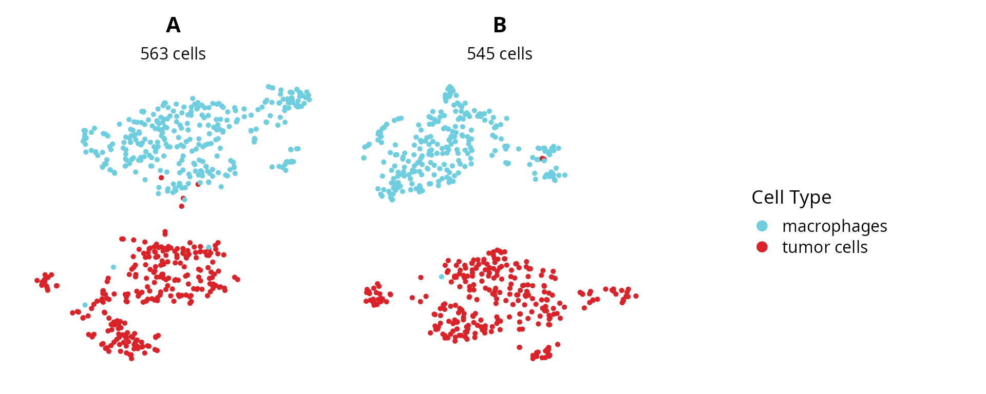
We annotate the cells to keep:
sobj_list = lapply(sobj_list, FUN = function(one_sobj) {
  one_sobj$is_of_interest = (one_sobj$cell_type %in% cell_type_of_interest)

  return(one_sobj)
})

lapply(sobj_list, FUN = function(one_sobj) {
  return(table(one_sobj$is_of_interest))
}) %>% do.call(rbind, .) %>%
  rbind(., colSums(.))
## FALSE TRUE
## A 308 255
## B 261 284
## 569 539Method 2: smoothed cluster annotation
We smooth cell type annotation at a cluster level:
sobj_list = lapply(sobj_list, FUN = function(one_sobj) {
  cluster_type = table(one_sobj$cell_type, one_sobj$seurat_clusters) %>%
    prop.table(., margin = 2) %>%
    apply(., 2, which.max)
  cluster_type = setNames(nm = names(cluster_type),
                          levels(one_sobj$cell_type)[cluster_type])

  one_sobj$cluster_type = setNames(nm = names(one_sobj$seurat_clusters),
                                   cluster_type[one_sobj$seurat_clusters])

  ## Output
  return(one_sobj)
})
We visualize the score for the cell type of interest, the cell type annotation, the clustering, and the cluster annotation.
plot_list = lapply(sobj_list, FUN = function(one_sobj) {
  project_name = as.character(unique(one_sobj$orig.ident))
  plot_sublist = list()

  # Score
  the_score = paste0("score_", gsub(x = cell_type_of_interest,
                                    pattern = " ",
                                    replacement = "_"))
  plot_sublist[[1]] = Seurat::FeaturePlot(one_sobj, reduction = name2D,
                                          features = the_score) +
    ggplot2::labs(title = project_name,
                  subtitle = the_score) +
    Seurat::NoAxes() +
    ggplot2::scale_color_gradientn(colors = aquarius:::palette_GrOrBl) +
    ggplot2::theme(aspect.ratio = 1,
                   plot.subtitle = element_text(hjust = 0.5))

  # Cell type
  plot_sublist[[2]] = Seurat::DimPlot(one_sobj,
                                      reduction = name2D,
                                      group.by = "cell_type",
                                      cols = color_markers) +
    ggplot2::labs(title = "Cell type annotation",
                  subtitle = paste0(sum(one_sobj$cell_type %in% cell_type_of_interest),
                                    " cells")) +
    Seurat::NoAxes() + Seurat::NoLegend() +
    ggplot2::theme(aspect.ratio = 1,
                   plot.title = element_text(hjust = 0.5),
                   plot.subtitle = element_text(hjust = 0.5))

  # Clusters
  plot_sublist[[3]] = Seurat::DimPlot(one_sobj,
                                      reduction = name2D,
                                      group.by = "seurat_clusters",
                                      label = TRUE) +
    ggplot2::labs(title = "Clusters") +
    Seurat::NoAxes() + Seurat::NoLegend() +
    ggplot2::theme(aspect.ratio = 1,
                   plot.title = element_text(hjust = 0.5),
                   plot.subtitle = element_text(hjust = 0.5))

  # Cluster type
  plot_sublist[[4]] = Seurat::DimPlot(one_sobj,
                                      reduction = name2D,
                                      group.by = "cluster_type",
                                      cols = color_markers) +
    ggplot2::labs(title = "Cluster annotation",
                  subtitle = paste0(sum(one_sobj$cluster_type %in% cell_type_of_interest),
                                    " cells")) +
    Seurat::NoAxes() + Seurat::NoLegend() +
    ggplot2::theme(aspect.ratio = 1,
                   plot.title = element_text(hjust = 0.5),
                   plot.subtitle = element_text(hjust = 0.5))

  return(plot_sublist)
}) %>% unlist(., recursive = FALSE)

patchwork::wrap_plots(plot_list, ncol = 4)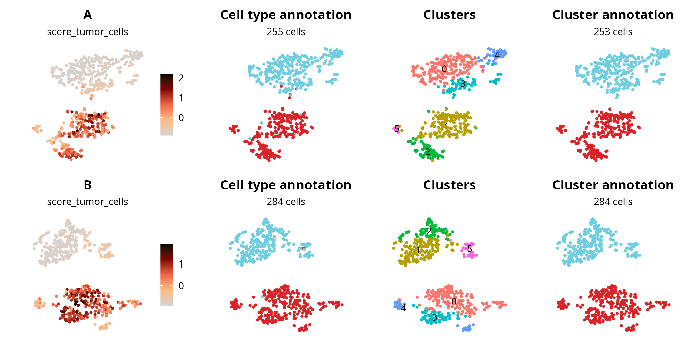
We annotate the cells to keep:
sobj_list = lapply(sobj_list, FUN = function(one_sobj) {
  one_sobj$is_of_interest = (one_sobj$cluster_type %in% cell_type_of_interest)

  return(one_sobj)
})

lapply(sobj_list, FUN = function(one_sobj) {
  return(table(one_sobj$is_of_interest))
}) %>% do.call(rbind, .) %>%
  rbind(., colSums(.))
## FALSE TRUE
## A 310 253
## B 261 284
## 571 537Method 3: average gene expression levels
We define a set of markers of interest. Here, we provide the exact same genes used for the cell type annotation. But, custom gene sets can be provided.
markers_of_interest = c("Sox9", "Sox10", "Ank3", "Plp1", "Col16a1")We attribute a score for each cell:
sobj_list = lapply(sobj_list, FUN = function(one_sobj) {
  one_sobj$score_of_interest = Seurat::AddModuleScore(one_sobj,
                                                      features = list(markers_of_interest))$Cluster1

  return(one_sobj)
})
We set an arbitrary threshold for the score:
score_thresh = 0.2We visualize the score, the cells with a score above the threshold, the clustering, and the average score by cluster.
plot_list = lapply(sobj_list, FUN = function(one_sobj) {
  project_name = as.character(unique(one_sobj$orig.ident))
  plot_sublist = list()

  # Score
  plot_sublist[[1]] = Seurat::FeaturePlot(one_sobj, reduction = name2D,
                                          features = "score_of_interest") +
    ggplot2::labs(title = project_name,
                  subtitle = "Score for genes of interest") +
    Seurat::NoAxes() +
    ggplot2::scale_color_gradientn(colors = aquarius:::palette_GrOrBl) +
    ggplot2::theme(aspect.ratio = 1,
                   plot.subtitle = element_text(hjust = 0.5))

  # Cells with high score
  one_sobj$score_above_threshold = (one_sobj$score_of_interest > score_thresh)
  plot_sublist[[2]] = Seurat::DimPlot(one_sobj,
                                      reduction = name2D,
                                      group.by = "score_above_threshold") +
    ggplot2::labs(title = paste0("Score thresold: ", score_thresh),
                  subtitle = paste0(sum(one_sobj$score_above_threshold), " cells")) +
    Seurat::NoAxes() + Seurat::NoLegend() +
    ggplot2::theme(aspect.ratio = 1,
                   plot.title = element_text(hjust = 0.5),
                   plot.subtitle = element_text(hjust = 0.5))

  # Clusters
  plot_sublist[[3]] = Seurat::DimPlot(one_sobj,
                                      reduction = name2D,
                                      group.by = "seurat_clusters",
                                      label = TRUE) +
    ggplot2::labs(title = "Clusters") +
    Seurat::NoAxes() + Seurat::NoLegend() +
    ggplot2::theme(aspect.ratio = 1,
                   plot.title = element_text(hjust = 0.5),
                   plot.subtitle = element_text(hjust = 0.5))

  # Score by cluster
  score_by_clusters = one_sobj@meta.data %>%
    dplyr::select(seurat_clusters, score_of_interest) %>%
    dplyr::group_by(seurat_clusters) %>%
    dplyr::summarise(avg_score = mean(score_of_interest)) %>%
    as.data.frame()

  clusters_high_score = score_by_clusters %>%
    dplyr::filter(avg_score > score_thresh) %>%
    dplyr::pull(seurat_clusters)
  nb_cells_in_clusters = sum(one_sobj$seurat_clusters %in% clusters_high_score)

  plot_sublist[[4]] = ggplot2::ggplot(score_by_clusters, aes(x = seurat_clusters, y = avg_score)) +
    ggplot2::geom_point() +
    ggplot2::geom_hline(yintercept = score_thresh, col = "red") +
    ggplot2::labs(x = "Cluster ID", y = "Mean score",
                  title = paste0("Score thresold: ", score_thresh),
                  subtitle = paste0(nb_cells_in_clusters, " cells")) +
    ggplot2::theme_classic() +
    ggplot2::theme(plot.title = element_text(hjust = 0.5, face = "bold"),
                   plot.subtitle = element_text(hjust = 0.5))

  return(plot_sublist)
}) %>% unlist(., recursive = FALSE)

patchwork::wrap_plots(plot_list, ncol = 4)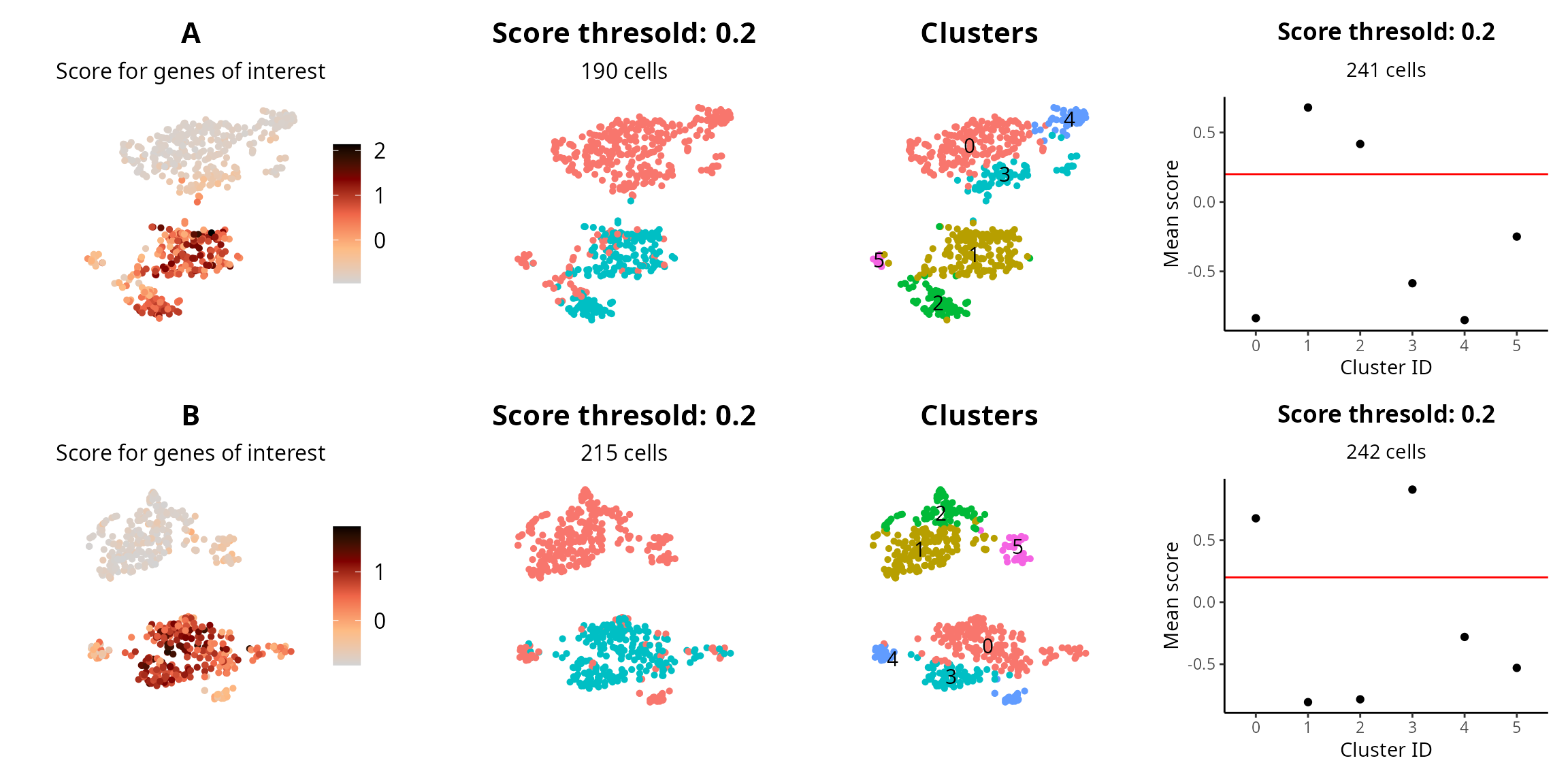
We annotate the cells to keep, based on the single-cell level score:
sobj_list = lapply(sobj_list, FUN = function(one_sobj) {
  one_sobj$is_of_interest = (one_sobj$score_of_interest > score_thresh)

  return(one_sobj)
})

lapply(sobj_list, FUN = function(one_sobj) {
  return(table(one_sobj$is_of_interest))
}) %>% do.call(rbind, .) %>%
  rbind(., colSums(.))
## FALSE TRUE
## A 373 190
## B 330 215
## 703 405Alternatively, based on the average score by cluster:
sobj_list = lapply(sobj_list, FUN = function(one_sobj) {
  clusters_high_score = one_sobj@meta.data %>%
    dplyr::select(seurat_clusters, score_of_interest) %>%
    dplyr::group_by(seurat_clusters) %>%
    dplyr::summarise(avg_score = mean(score_of_interest)) %>%
    dplyr::filter(avg_score > score_thresh) %>%
    dplyr::pull(seurat_clusters)

  one_sobj$is_of_interest = (one_sobj$seurat_clusters %in% clusters_high_score)

  return(one_sobj)
})

lapply(sobj_list, FUN = function(one_sobj) {
  return(table(one_sobj$is_of_interest))
}) %>% do.call(rbind, .) %>%
  rbind(., colSums(.))
## FALSE TRUE
## A 322 241
## B 303 242
## 625 483Combined dataset
For this example, we extract cells based on the cluster-smoothed cell type annotation.
sobj_list = lapply(sobj_list, FUN = function(one_sobj) {
  one_sobj$is_of_interest = (one_sobj$cluster_type %in% cell_type_of_interest)

  return(one_sobj)
})

lapply(sobj_list, FUN = function(one_sobj) {
  return(table(one_sobj$is_of_interest))
}) %>% do.call(rbind, .) %>%
  rbind(., colSums(.))
## FALSE TRUE
## A 310 253
## B 261 284
## 571 537We subset the individual objects:
sobj_list = lapply(sobj_list, FUN = function(one_sobj) {
  if (sum(one_sobj$is_of_interest) > 0) {
    one_sobj = subset(one_sobj, is_of_interest == TRUE)
  } else {
    one_sobj = NA
  }
  return(one_sobj)
})

lapply(sobj_list, FUN = dim) %>%
  do.call(rbind, .) %>%
  rbind(., colSums(.)) %>%
  `colnames<-`(c("Nb genes", "Nb cells"))
## Nb genes Nb cells
## A 28000 253
## B 28000 284
## 56000 537We combine the dataset:
sobj = base::merge(sobj_list[[1]],
                   y = sobj_list[c(2:length(sobj_list))],
                   add.cell.ids = names(sobj_list))
sobj
## An object of class Seurat
## 28000 features across 537 samples within 1 assay
## Active assay: RNA (28000 features, 3000 variable features)
## 6 layers present: counts.A, counts.B, data.A, scale.data.A, data.B, scale.data.BWe merge the layers:
sobj = SeuratObject::JoinLayers(sobj, layers = "counts")
sobj = SeuratObject::JoinLayers(sobj, layers = "data")
sobj = SeuratObject::JoinLayers(sobj, layers = "scale.data")

sobj
## An object of class Seurat
## 28000 features across 537 samples within 1 assay
## Active assay: RNA (28000 features, 3000 variable features)
## 3 layers present: scale.data, data, countsWe add again the correspondence between gene names and gene ID. Since all datasets have been aligned using the same transcriptome, we take the correspondence from one individual dataset.
sobj@assays$RNA@meta.data = sobj_list[[1]]@assays$RNA@meta.data[, c("Ensembl_ID", "gene_name")]

head(sobj@assays$RNA@meta.data)
## Ensembl_ID gene_name
## Xkr4 ENSMUSG00000051951 Xkr4
## Gm1992 ENSMUSG00000089699 Gm1992
## Gm37381 ENSMUSG00000102343 Gm37381
## Rp1 ENSMUSG00000025900 Rp1
## Rp1.1 ENSMUSG00000109048 Rp1
## Sox17 ENSMUSG00000025902 Sox17We remove the list of objects:
rm(sobj_list)What is are the cells metadata ?
sobj$is_of_interest = NULL
sobj$score_of_interest = NULL

summary(sobj@meta.data)
## orig.ident nCount_RNA nFeature_RNA log_nCount_RNA
## Length:537 Min. : 1022 Min. : 601 Min. : 6.930
## Class :character 1st Qu.: 2349 1st Qu.:1056 1st Qu.: 7.762
## Mode :character Median : 3878 Median :1667 Median : 8.263
## Mean : 5792 Mean :2011 Mean : 8.351
## 3rd Qu.: 6666 3rd Qu.:2553 3rd Qu.: 8.805
## Max. :33763 Max. :6042 Max. :10.427
## Seurat.Phase cyclone.Phase RNA_snn_res.0.5 seurat_clusters
## Length:537 Length:537 Length:537 Length:537
## Class :character Class :character Class :character Class :character
## Mode :character Mode :character Mode :character Mode :character
##
##
##
## percent.mt percent.rb score_macrophages score_tumor_cells
## Min. : 0.000 Min. : 0.1894 Min. :-1.2490 Min. :-0.7305
## 1st Qu.: 5.643 1st Qu.: 1.1910 1st Qu.:-1.0310 1st Qu.: 0.1883
## Median :10.242 Median : 3.0620 Median :-0.8385 Median : 0.6353
## Mean :10.559 Mean : 4.8629 Mean :-0.8324 Mean : 0.5720
## 3rd Qu.:15.902 3rd Qu.: 7.2975 3rd Qu.:-0.6642 3rd Qu.: 0.9543
## Max. :19.959 Max. :19.9397 Max. : 0.9580 Max. : 2.2151
## cell_type cluster_type
## Length:537 Length:537
## Class :character Class :character
## Mode :character Mode :character
##
##
## Processing
We remove genes that are expressed in less than 5 cells:
sobj = aquarius::filter_features(sobj, min_cells = 5)
sobj
## An object of class Seurat
## 12361 features across 537 samples within 1 assay
## Active assay: RNA (12361 features, 0 variable features)
## 3 layers present: scale.data, data, countsProjection
We normalize the count matrix for remaining cells and select highly variable features:
sobj = Seurat::NormalizeData(sobj,
                             normalization.method = "LogNormalize")
sobj = Seurat::FindVariableFeatures(sobj, nfeatures = 2000)
sobj = Seurat::ScaleData(sobj)

sobj
## An object of class Seurat
## 12361 features across 537 samples within 1 assay
## Active assay: RNA (12361 features, 2000 variable features)
## 3 layers present: scale.data, data, countsWe perform a PCA:
sobj = Seurat::RunPCA(sobj,
                      assay = "RNA",
                      reduction.name = "RNA_pca",
                      npcs = 100,
                      seed.use = 1337L)
sobj
## An object of class Seurat
## 12361 features across 537 samples within 1 assay
## Active assay: RNA (12361 features, 2000 variable features)
## 3 layers present: scale.data, data, counts
## 1 dimensional reduction calculated: RNA_pcaWe choose the number of dimensions such that they summarize 60 % of the variability:
stdev = sobj@reductions[["RNA_pca"]]@stdev
stdev_prop = cumsum(stdev)/sum(stdev)
ndims = which(stdev_prop > 0.60)[1]
ndims
## [1] 51We can visualize this on the elbow plot:
elbow_p = Seurat::ElbowPlot(sobj, ndims = 100, reduction = "RNA_pca") +
  ggplot2::geom_point(x = ndims, y = stdev[ndims], col = "red")
x_text = ggplot_build(elbow_p)$layout$panel_params[[1]]$x$get_labels() %>% as.numeric()
elbow_p = elbow_p +
  ggplot2::scale_x_continuous(breaks = sort(c(x_text, ndims)), limits = c(0, 100))
x_color = ifelse(ggplot_build(elbow_p)$layout$panel_params[[1]]$x$get_labels() %>%
                   as.numeric() %>% round(., 2) == round(ndims, 2), "red", "black")
elbow_p = elbow_p +
  ggplot2::theme_classic() +
  ggplot2::theme(axis.text.x = element_text(color = x_color))

elbow_p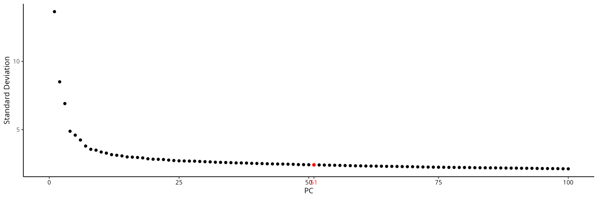
We generate a tSNE and a UMAP with 51 principal components:
sobj = Seurat::RunTSNE(sobj,
                       reduction = "RNA_pca",
                       dims = 1:ndims,
                       seed.use = 1337L,
                       num_threads = n_threads, # Rtsne::Rtsne option
                       reduction.name = paste0("RNA_pca_", ndims, "_tsne"))

sobj = Seurat::RunUMAP(sobj,
                       reduction = "RNA_pca",
                       dims = 1:ndims,
                       seed.use = 1337L,
                       reduction.name = paste0("RNA_pca_", ndims, "_umap"))
(Time to run: 3.74 s)
We can visualize the two representations:
tsne = Seurat::DimPlot(sobj, group.by = "orig.ident",
                       reduction = paste0("RNA_pca_", ndims, "_tsne")) +
  ggplot2::scale_color_manual(values = sample_info$color,
                              breaks = sample_info$project_name) +
  Seurat::NoAxes() + ggplot2::ggtitle("PCA - tSNE") +
  ggplot2::theme(aspect.ratio = 1,
                 plot.title = element_text(hjust = 0.5),
                 legend.position = "none")

umap = Seurat::DimPlot(sobj, group.by = "orig.ident",
                       reduction = paste0("RNA_pca_", ndims, "_umap")) +
  ggplot2::scale_color_manual(values = sample_info$color,
                              breaks = sample_info$project_name) +
  Seurat::NoAxes() + ggplot2::ggtitle("PCA - UMAP") +
  ggplot2::theme(aspect.ratio = 1,
                 plot.title = element_text(hjust = 0.5))

tsne | umap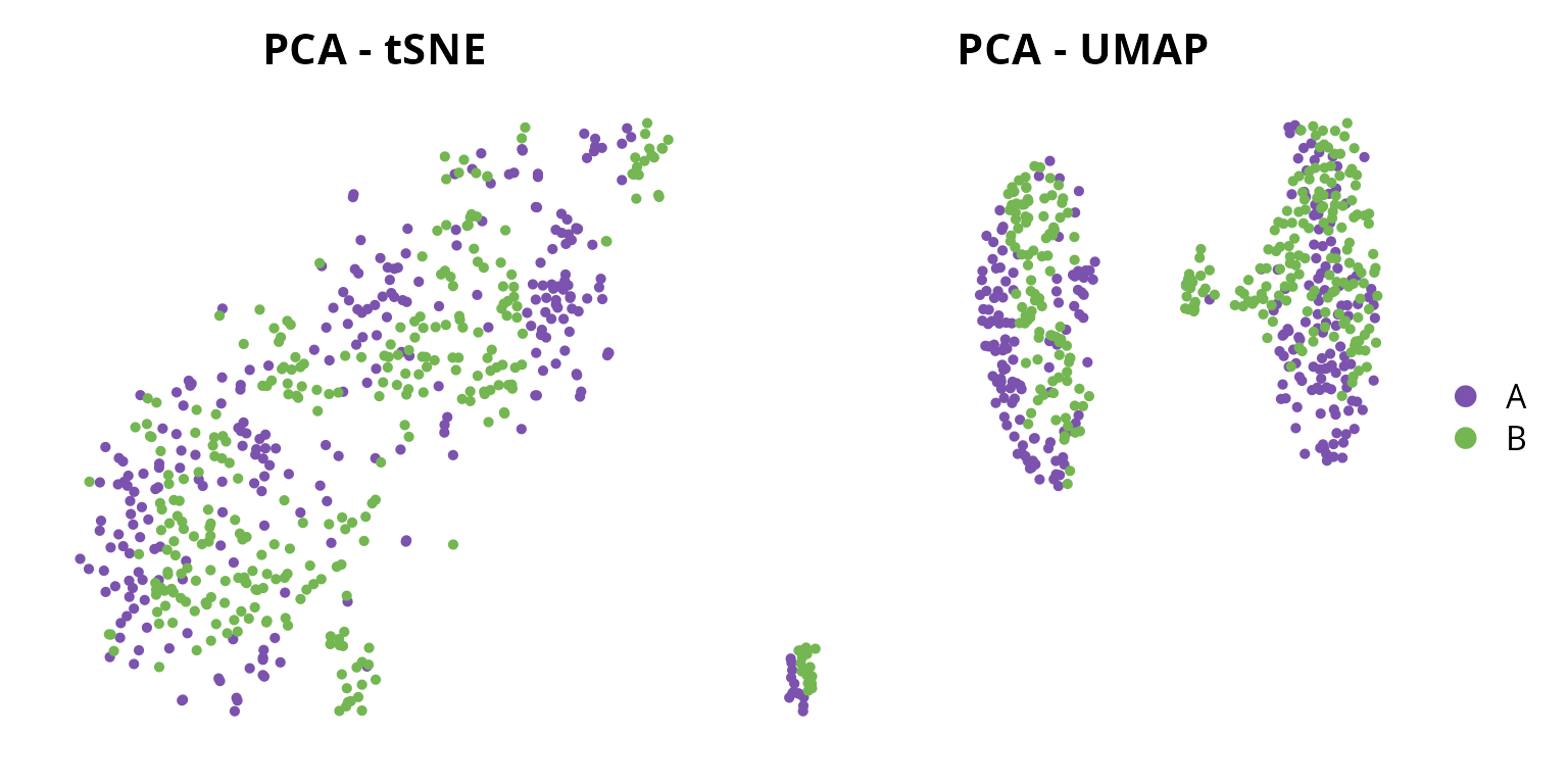
Batch-effect correction
We remove sample specific effect on the pca using
FastMNN:
sobj = aquarius::integration_fastmnn(sobj = sobj,
                                     split_by = "orig.ident",
                                     assay = "RNA",
                                     verbose = TRUE,
                                     d = 100)

sobj
## An object of class Seurat
## 14361 features across 537 samples within 2 assays
## Active assay: RNA (12361 features, 2000 variable features)
## 3 layers present: scale.data, data, counts
## 1 other assay present: mnn.reconstructed
## 4 dimensional reductions calculated: RNA_pca, RNA_pca_51_tsne, RNA_pca_51_umap, mnn(Time to run: 6.89 s)
From this batch-effect removed projection, we generate a tSNE and a UMAP.
sobj = Seurat::RunUMAP(sobj,
                       seed.use = 1337L,
                       dims = 1:ndims,
                       reduction = "mnn",
                       reduction.name = paste0("mnn_", ndims, "_umap"),
                       reduction.key = paste0("mnn_", ndims, "umap_"))

sobj = Seurat::RunTSNE(sobj,
                       dims = 1:ndims,
                       seed.use = 1337L,
                       num_threads = n_threads, # Rtsne::Rtsne option
                       reduction = "mnn",
                       reduction.name = paste0("mnn_", ndims, "_tsne"),
                       reduction.key = paste0("mnn", ndims, "tsne_"))
(Time to run: 3.88 s)
We visualize the corrected projections:
tsne = Seurat::DimPlot(sobj, group.by = "orig.ident",
                       reduction = paste0("mnn_", ndims, "_tsne")) +
  ggplot2::scale_color_manual(values = sample_info$color,
                              breaks = sample_info$project_name) +
  Seurat::NoAxes() + ggplot2::ggtitle("PCA - mnn - tSNE") +
  ggplot2::theme(aspect.ratio = 1,
                 plot.title = element_text(hjust = 0.5),
                 legend.position = "none")

umap = Seurat::DimPlot(sobj, group.by = "orig.ident",
                       reduction = paste0("mnn_", ndims, "_umap")) +
  ggplot2::scale_color_manual(values = sample_info$color,
                              breaks = sample_info$project_name) +
  Seurat::NoAxes() + ggplot2::ggtitle("PCA - mnn - UMAP") +
  ggplot2::theme(aspect.ratio = 1,
                 plot.title = element_text(hjust = 0.5))

tsne | umap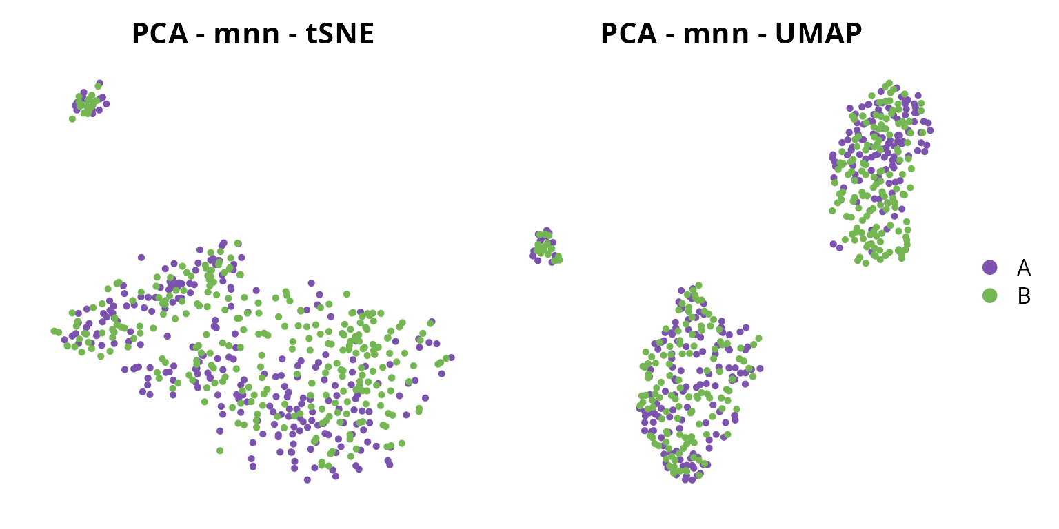
Diffusion map
We generate a diffusion map from the batch-effect corrected space:
reduction_name = "mnn"

sobj = aquarius::run_diffusion_map(sobj = sobj,
                                   input = reduction_name,
                                   n_eigs = 50)
sobj
## An object of class Seurat
## 14361 features across 537 samples within 2 assays
## Active assay: RNA (12361 features, 2000 variable features)
## 3 layers present: scale.data, data, counts
## 1 other assay present: mnn.reconstructed
## 7 dimensional reductions calculated: RNA_pca, RNA_pca_51_tsne, RNA_pca_51_umap, mnn, mnn_51_umap, mnn_51_tsne, mnn_dmWe visualize it:
dm_name = paste0(reduction_name, "_dm")

Seurat::DimPlot(sobj, reduction = dm_name,
                group.by = "orig.ident") +
  ggplot2::scale_color_manual(values = sample_info$color,
                              breaks = sample_info$sample_identifiant) +
  ggplot2::labs(title = dm_name) +
  ggplot2::theme(aspect.ratio = 1,
                 plot.title = element_text(hjust = 0.5)) +
  Seurat::NoAxes()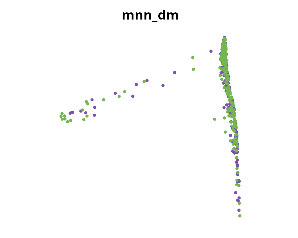
For visualisation, we keep the tSNE:
name2D = paste0("mnn_", ndims, "_tsne")Clustering
We generate a clustering:
sobj = Seurat::FindNeighbors(sobj, reduction = reduction_name, dims = 1:ndims)
sobj = Seurat::FindClusters(sobj, resolution = 0.5)
## Modularity Optimizer version 1.3.0 by Ludo Waltman and Nees Jan van Eck
##
## Number of nodes: 537
## Number of edges: 23208
##
## Running Louvain algorithm...
## Maximum modularity in 10 random starts: 0.7868
## Number of communities: 4
## Elapsed time: 0 seconds
clusters_plot = Seurat::DimPlot(sobj, reduction = name2D, label = TRUE) +
  Seurat::NoAxes() + Seurat::NoLegend() +
  ggplot2::labs(title = "Clusters ID") +
  ggplot2::theme(aspect.ratio = 1,
                 plot.title = element_text(hjust = 0.5))
clusters_plot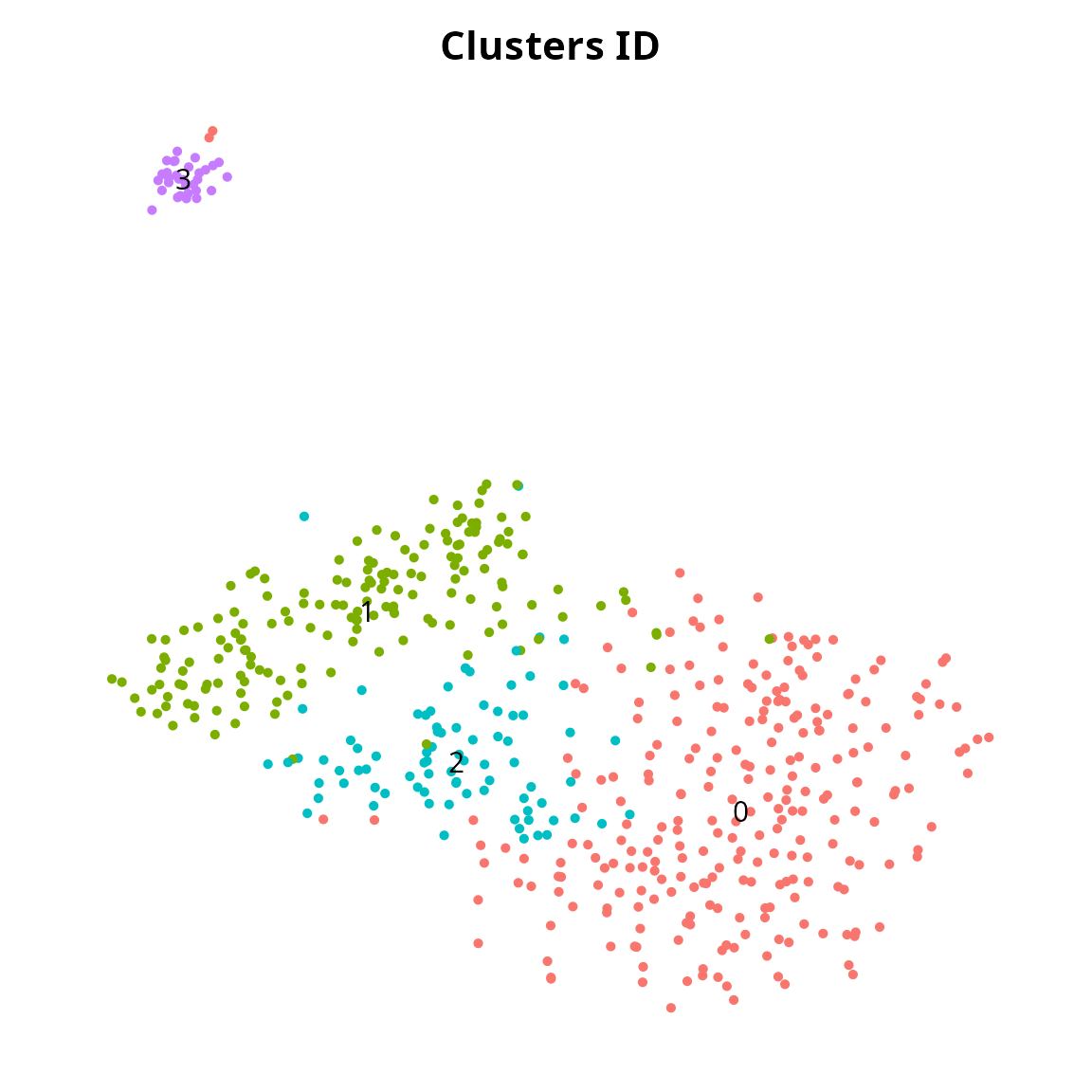
Visualization
We represent the 4 quality metrics:
plot_list = Seurat::FeaturePlot(sobj, reduction = name2D,
                                combine = FALSE, pt.size = 0.25,
                                features = c("percent.mt", "percent.rb", "log_nCount_RNA", "nFeature_RNA"))
plot_list = lapply(plot_list, FUN = function(one_plot) {
  one_plot +
    Seurat::NoAxes() +
    ggplot2::scale_color_gradientn(colors = aquarius::palette_GrOrBl) +
    ggplot2::theme(aspect.ratio = 1)
})

patchwork::wrap_plots(plot_list, nrow = 1)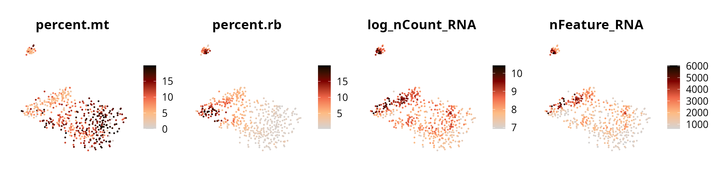
R Session
show
## R version 4.4.3 (2025-02-28)
## Platform: x86_64-pc-linux-gnu
## Running under: Ubuntu 24.10
##
## Matrix products: default
## BLAS:   /usr/lib/x86_64-linux-gnu/blas/libblas.so.3.12.0
## LAPACK: /usr/lib/x86_64-linux-gnu/lapack/liblapack.so.3.12.0
##
## locale:
##  [1] LC_CTYPE=en_US.UTF-8       LC_NUMERIC=C
##  [3] LC_TIME=fr_FR.UTF-8        LC_COLLATE=en_US.UTF-8
##  [5] LC_MONETARY=fr_FR.UTF-8    LC_MESSAGES=en_US.UTF-8
##  [7] LC_PAPER=fr_FR.UTF-8       LC_NAME=C
##  [9] LC_ADDRESS=C               LC_TELEPHONE=C
## [11] LC_MEASUREMENT=fr_FR.UTF-8 LC_IDENTIFICATION=C
##
## time zone: Europe/Paris
## tzcode source: system (glibc)
##
## attached base packages:
## [1] stats     graphics  grDevices utils     datasets  methods   base
##
## other attached packages:
## [1] future_1.40.0   ggplot2_3.5.2   patchwork_1.3.0 dplyr_1.1.4
##
## loaded via a namespace (and not attached):
##   [1] RcppAnnoy_0.0.22            splines_4.4.3
##   [3] later_1.4.2                 batchelor_1.22.0
##   [5] tibble_3.2.1                polyclip_1.10-7
##   [7] xts_0.14.1                  fastDummies_1.7.5
##   [9] lifecycle_1.0.4             doParallel_1.0.17
##  [11] globals_0.17.0              lattice_0.22-6
##  [13] MASS_7.3-65                 vcd_1.4-13
##  [15] magrittr_2.0.3              plotly_4.10.4
##  [17] sass_0.4.10                 rmarkdown_2.29
##  [19] jquerylib_0.1.4             yaml_2.3.10
##  [21] httpuv_1.6.16               Seurat_5.3.0
##  [23] sctransform_0.4.2           spam_2.11-1
##  [25] sp_2.2-0                    spatstat.sparse_3.1-0
##  [27] reticulate_1.42.0           cowplot_1.1.3
##  [29] pbapply_1.7-2               RColorBrewer_1.1-3
##  [31] ResidualMatrix_1.16.0       abind_1.4-8
##  [33] zlibbioc_1.52.0             Rtsne_0.17
##  [35] GenomicRanges_1.58.0        purrr_1.0.4
##  [37] BiocGenerics_0.52.0         nnet_7.3-20
##  [39] circlize_0.4.16             GenomeInfoDbData_1.2.13
##  [41] IRanges_2.40.1              S4Vectors_0.44.0
##  [43] ggrepel_0.9.6               irlba_2.3.5.1
##  [45] listenv_0.9.1               spatstat.utils_3.1-3
##  [47] goftest_1.2-3               RSpectra_0.16-2
##  [49] spatstat.random_3.3-3       fitdistrplus_1.2-2
##  [51] parallelly_1.43.0           pkgdown_2.1.2
##  [53] DelayedMatrixStats_1.28.1   smoother_1.3
##  [55] codetools_0.2-20            DelayedArray_0.32.0
##  [57] scuttle_1.16.0              tidyselect_1.2.1
##  [59] shape_1.4.6.1               UCSC.utils_1.2.0
##  [61] farver_2.1.2                ScaledMatrix_1.14.0
##  [63] matrixStats_1.5.0           stats4_4.4.3
##  [65] spatstat.explore_3.4-2      jsonlite_2.0.0
##  [67] GetoptLong_1.0.5            BiocNeighbors_2.0.1
##  [69] e1071_1.7-16                Formula_1.2-5
##  [71] progressr_0.15.1            ggridges_0.5.6
##  [73] survival_3.8-3              iterators_1.0.14
##  [75] systemfonts_1.2.3           foreach_1.5.2
##  [77] tools_4.4.3                 ragg_1.4.0
##  [79] ica_1.0-3                   Rcpp_1.0.14
##  [81] glue_1.8.0                  gridExtra_2.3
##  [83] SparseArray_1.6.2           ranger_0.17.0
##  [85] laeken_0.5.3                xfun_0.52
##  [87] TTR_0.24.4                  MatrixGenerics_1.18.1
##  [89] ggthemes_5.1.0              GenomeInfoDb_1.42.3
##  [91] withr_3.0.2                 fastmap_1.2.0
##  [93] boot_1.3-31                 VIM_6.2.2
##  [95] digest_0.6.37               rsvd_1.0.5
##  [97] R6_2.6.1                    mime_0.13
##  [99] textshaping_1.0.1           colorspace_2.1-1
## [101] scattermore_1.2             tensor_1.5
## [103] spatstat.data_3.1-6         hexbin_1.28.5
## [105] tidyr_1.3.1                 generics_0.1.3
## [107] data.table_1.17.0           robustbase_0.99-4-1
## [109] class_7.3-23                httr_1.4.7
## [111] htmlwidgets_1.6.4           S4Arrays_1.6.0
## [113] scatterplot3d_0.3-44        uwot_0.2.3
## [115] pkgconfig_2.0.3             gtable_0.3.6
## [117] ComplexHeatmap_2.23.1       lmtest_0.9-40
## [119] SingleCellExperiment_1.28.1 XVector_0.46.0
## [121] destiny_3.20.0              htmltools_0.5.8.1
## [123] carData_3.0-5               dotCall64_1.2
## [125] clue_0.3-66                 SeuratObject_5.1.0
## [127] scales_1.4.0                Biobase_2.66.0
## [129] png_0.1-8                   knn.covertree_1.0
## [131] spatstat.univar_3.1-2       knitr_1.50
## [133] reshape2_1.4.4              rjson_0.2.23
## [135] curl_6.2.2                  aquarius_1.0.0
## [137] nlme_3.1-168                proxy_0.4-27
## [139] cachem_1.1.0                zoo_1.8-14
## [141] GlobalOptions_0.1.2         stringr_1.5.1
## [143] KernSmooth_2.23-26          parallel_4.4.3
## [145] miniUI_0.1.2                desc_1.4.3
## [147] pillar_1.10.2               grid_4.4.3
## [149] vctrs_0.6.5                 pcaMethods_1.98.0
## [151] RANN_2.6.2                  promises_1.3.2
## [153] car_3.1-3                   BiocSingular_1.22.0
## [155] beachmat_2.22.0             xtable_1.8-4
## [157] cluster_2.1.8.1             evaluate_1.0.3
## [159] cli_3.6.5                   compiler_4.4.3
## [161] rlang_1.1.6                 crayon_1.5.3
## [163] future.apply_1.11.3         labeling_0.4.3
## [165] plyr_1.8.9                  fs_1.6.6
## [167] stringi_1.8.7               viridisLite_0.4.2
## [169] deldir_2.0-4                BiocParallel_1.40.2
## [171] lazyeval_0.2.2              spatstat.geom_3.3-6
## [173] Matrix_1.7-3                RcppHNSW_0.6.0
## [175] RcppEigen_0.3.4.0.2         sparseMatrixStats_1.18.0
## [177] shiny_1.10.0                SummarizedExperiment_1.36.0
## [179] ROCR_1.0-11                 igraph_2.1.4
## [181] bslib_0.9.0                 DEoptimR_1.1-3-1
## [183] ggplot.multistats_1.0.1