The goal of this script is to make figure to show how to use the
functions from aquarius.
## [1] "/usr/lib/R/library"            "/usr/local/lib/R/site-library"
## [3] "/usr/lib/R/site-library"
Preparation
We load the dataset:
sobj = readRDS("./2_combined/combined_sobj.rds")
sobj
## An object of class Seurat
## 13774 features across 1108 samples within 1 assay
## Active assay: RNA (13774 features, 2000 variable features)
## 3 layers present: scale.data, data, counts
## 6 dimensional reductions calculated: RNA_pca, RNA_pca_48_tsne, RNA_pca_48_umap, harmony, harmony_48_umap, harmony_48_tsneHere are custom colors for each cell type:
color_markers = c("macrophages" = "#6ECEDF",
                  "tumor cells" = "#DA2328")
We define custom colors for each sample:
sample_info = data.frame(
  project_name = c("A", "B"),
  sample_identifier = c("A", "B"),
  color = c("#7B52AE", "#74B652"),
  row.names = c("A", "B"))

aquarius::plot_df(sample_info)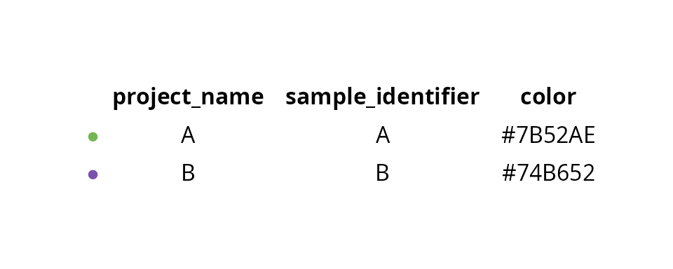
Visualization
Each section is named by the function it refers to.
plot_alluvial
We want to visualize the changes between a single-cell level cell type annotation and the annotation smoothed at a cluster level. Before making the figure, we smooth the annotation.
sobj$cell_type = factor(sobj$cell_type, levels = names(color_markers))

cluster_type = table(sobj$cell_type, sobj$seurat_clusters) %>%
  prop.table(., margin = 2) %>%
  apply(., 2, which.max)
cluster_type = setNames(nm = names(cluster_type),
                        levels(sobj$cell_type)[cluster_type])

sobj$cluster_type = setNames(nm = colnames(sobj),
                             cluster_type[sobj$seurat_clusters])
sobj$cluster_type = factor(sobj$cluster_type, levels = names(color_markers))
The alluvial plot shows how the annotation of cells changes between the two methods.
aquarius::plot_alluvial(sobj@meta.data,
                        column1 = "cell_type",
                        column2 = "cluster_type",
                        colors = color_markers)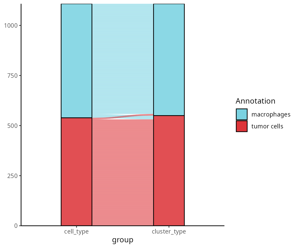
plot_c30_palette
We visualize the aquarius::c30_palette color
palette.
aquarius::plot_c30_palette()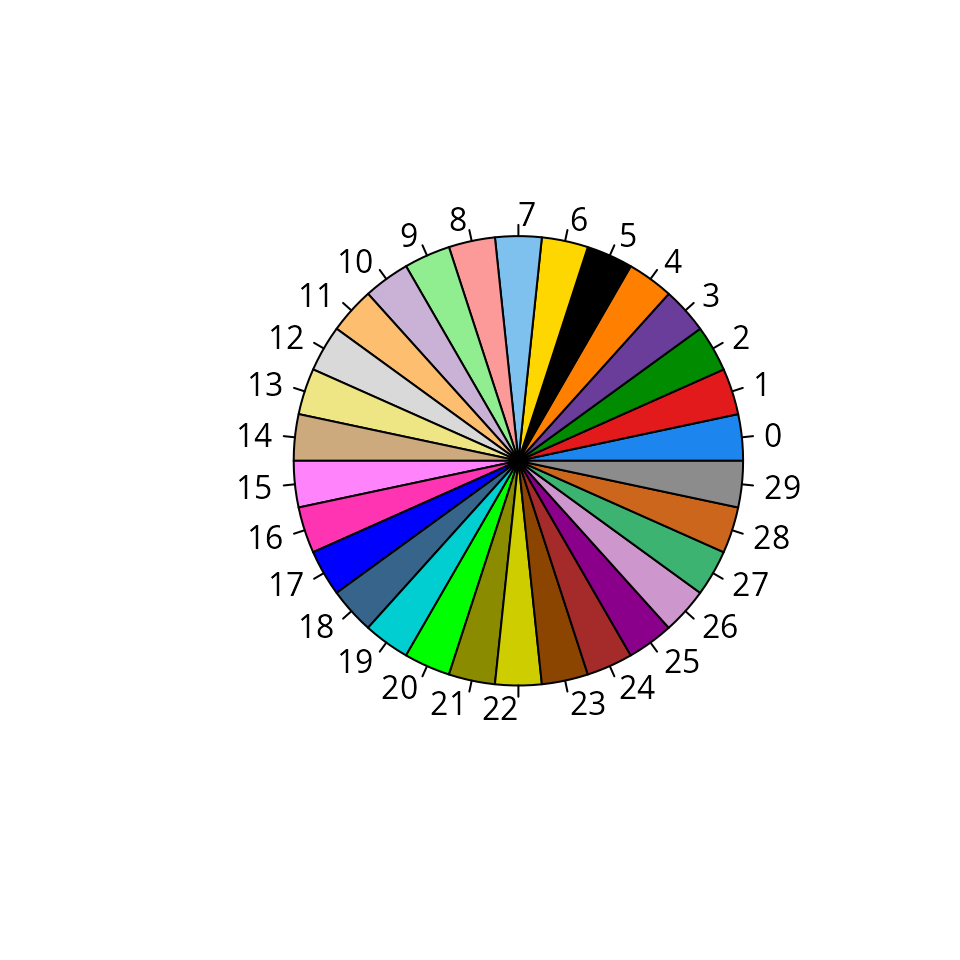
The colors are:
aquarius::c30_palette## [1] "dodgerblue2" "#E31A1C" "green4" "#6A3D9A"
## [5] "#FF7F00" "black" "gold1" "skyblue2"
## [9] "#FB9A99" "palegreen2" "#CAB2D6" "#FDBF6F"
## [13] "gray85" "khaki2" "burlywood3" "orchid1"
## [17] "maroon1" "blue1" "steelblue4" "darkturquoise"
## [21] "green1" "yellow4" "yellow3" "darkorange4"
## [25] "brown" "darkmagenta" "plum3" "mediumseagreen"
## [29] "chocolate3" "gray55"plot_piechart_subpopulation
aquarius::plot_piechart_subpopulation(
  sobj,
  reduction = "harmony_48_tsne",
  big_group_column = "cell_type",
  big_group_of_interest = "macrophages",
  big_group_color = color_markers[["macrophages"]],
  small_group_column = "seurat_clusters",
  composition_column = "orig.ident",
  composition_color = sample_info$color,
  bg_color = "gray92")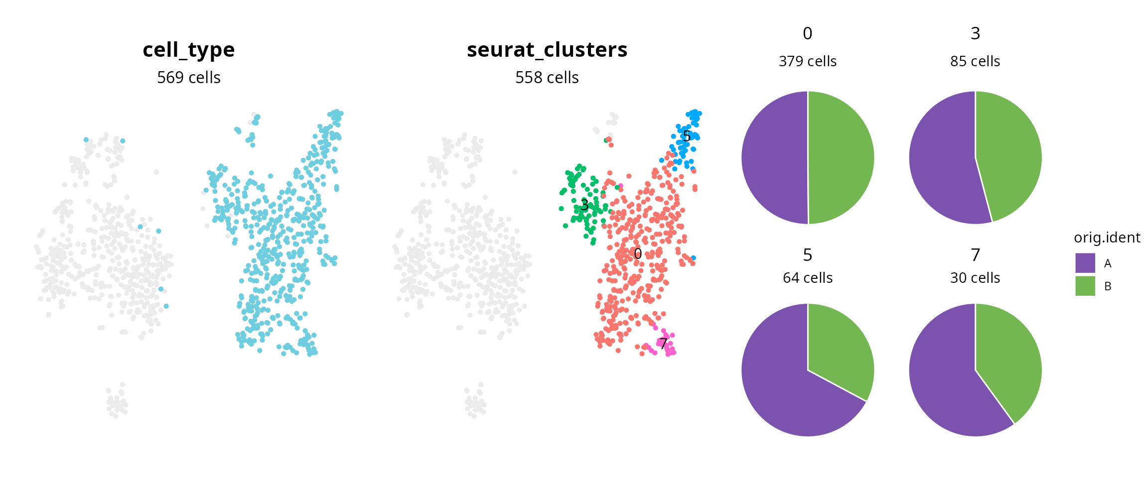
plot_subpopulation
Seurat::Idents(sobj) = sobj$cell_type

aquarius::plot_subpopulation(sobj,
                             reduction = "harmony_48_tsne",
                             identity = "tumor cells",
                             group_color = color_markers,
                             name_other = "other cells")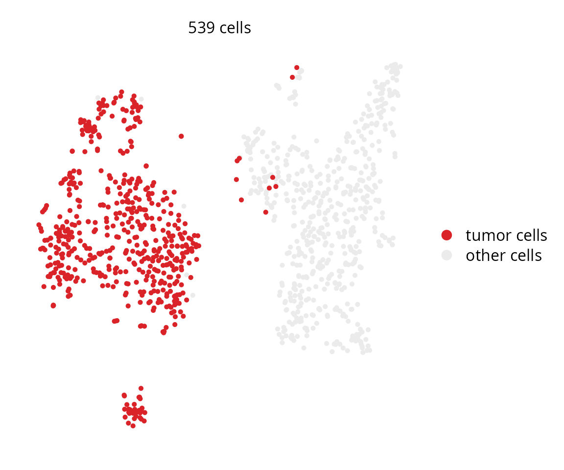
Other functions
Each section is named by the function it refers to.
print_to_copy_paste
A function to easily copy-paste a character vector:
my_vector = aquarius::c30_palette

aquarius::print_to_copy_paste(my_vector)
## dodgerblue2
## #E31A1C
## green4
## #6A3D9A
## #FF7F00
## black
## gold1
## skyblue2
## #FB9A99
## palegreen2
## #CAB2D6
## #FDBF6F
## gray85
## khaki2
## burlywood3
## orchid1
## maroon1
## blue1
## steelblue4
## darkturquoise
## green1
## yellow4
## yellow3
## darkorange4
## brown
## darkmagenta
## plum3
## mediumseagreen
## chocolate3
## gray55run_rescale
We consider a numerical vector:
df = data.frame(original = sobj$score_macrophages)

head(df)
## original
## A_"AAACCCATCAAGTCGT-1" -1.13779791
## A_"AAAGGTATCGTCTCAC-1" 0.96846694
## A_"AAAGTGACATCATTTC-1" 0.97000123
## A_"AAAGTGATCATGGAGG-1" -0.04234935
## A_"AACAAAGTCATTGTTC-1" 1.00857441
## A_"AACAAGAGTTTGATCG-1" 0.61423985We re-scale the distribution between -5 and 2, without keeping the 0 value at 0:
df$keep_zero_FALSE = aquarius::run_rescale(df$original,
                                           new_min = -5,
                                           new_max = 2,
                                           keep_zero = FALSE)

ggplot2::ggplot(df, aes(x = original, y = keep_zero_FALSE)) +
  ggplot2::geom_abline(slope = 1, intercept = 0, lty = 2, color = "gray") +
  ggplot2::geom_hline(yintercept = 0, color = "gray") +
  ggplot2::geom_vline(xintercept = 0, color = "gray") +
  ggplot2::labs(x = "Original values",
                y = "Rescaled values",
                title = "aquarius::run_rescale",
                subtitle = "with keep_zero = FALSE") +
  ggplot2::geom_point() +
  ggplot2::theme_classic() +
  ggplot2::theme(plot.title = element_text(hjust = 0.5),
                 plot.subtitle = element_text(hjust = 0.5),
                 panel.grid.major = element_line())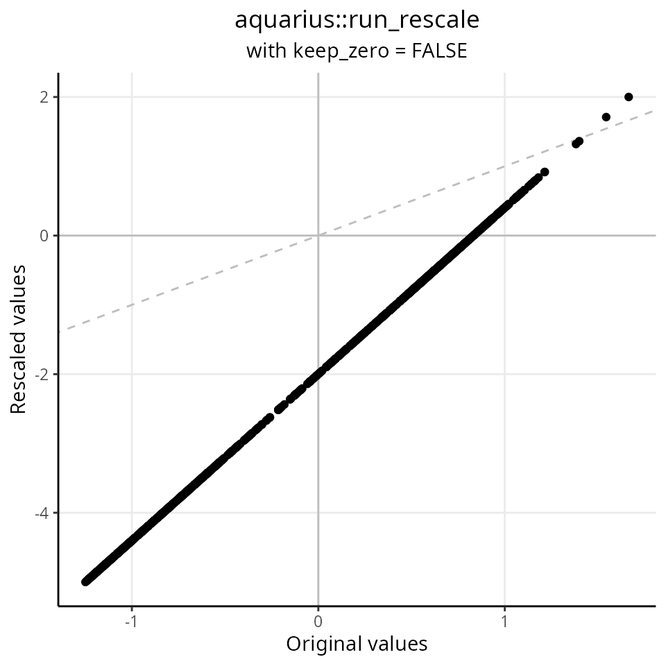
We re-scale the distribution between -5 and 2, with keeping the 0 value at 0:
df$keep_zero_TRUE = aquarius::run_rescale(df$original,
                                          new_min = -5,
                                          new_max = 2,
                                          keep_zero = TRUE)

ggplot2::ggplot(df, aes(x = original, y = keep_zero_TRUE)) +
  ggplot2::geom_abline(slope = 1, intercept = 0, lty = 2, color = "gray") +
  ggplot2::geom_hline(yintercept = 0, color = "gray") +
  ggplot2::geom_vline(xintercept = 0, color = "gray") +
  ggplot2::labs(x = "Original values",
                y = "Rescaled values",
                title = "aquarius::run_rescale",
                subtitle = "with keep_zero = TRUE") +
  ggplot2::geom_point() +
  ggplot2::theme_classic() +
  ggplot2::theme(plot.title = element_text(hjust = 0.5),
                 plot.subtitle = element_text(hjust = 0.5),
                 panel.grid.major = element_line())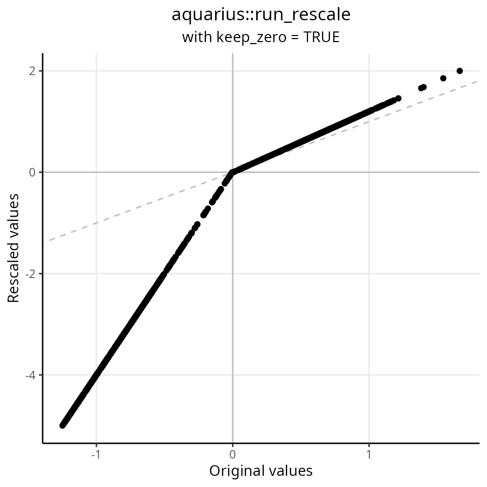
sample_cell_barcode
We visualize the clustering:
Seurat::DimPlot(sobj,
                reduction = "harmony_48_tsne",
                group.by = "seurat_clusters",
                label = TRUE) +
  Seurat::NoAxes() + Seurat::NoLegend() +
  ggplot2::theme(aspect.ratio = 1)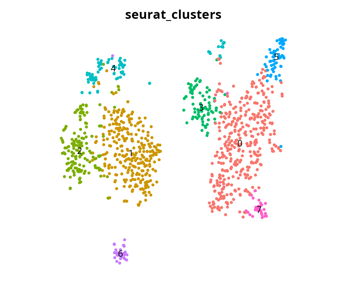
We subset a maximum of 10 cells per cluster:
Seurat::Idents(sobj) = sobj$seurat_clusters

subsobj = aquarius::sample_cell_barcode(sobj,
                                        n = 10)
subsobj
## An object of class Seurat
## 13774 features across 80 samples within 1 assay
## Active assay: RNA (13774 features, 2000 variable features)
## 3 layers present: scale.data, data, counts
## 6 dimensional reductions calculated: RNA_pca, RNA_pca_48_tsne, RNA_pca_48_umap, harmony, harmony_48_umap, harmony_48_tsneWe visualize the projection with the remaining cells:
Seurat::DimPlot(subsobj,
                reduction = "harmony_48_tsne",
                group.by = "seurat_clusters",
                label = TRUE) +
  Seurat::NoAxes() + Seurat::NoLegend() +
  ggplot2::theme(aspect.ratio = 1)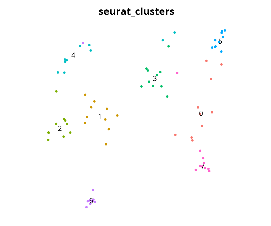
Cleaning :)
rm(subsobj)Functions to add
To be added in this vignette:
plot_externalread_gtfprepare_gsearepro_dependency_treerepro_installation_order
R Session
show
## R version 4.4.3 (2025-02-28)
## Platform: x86_64-pc-linux-gnu
## Running under: Ubuntu 24.10
##
## Matrix products: default
## BLAS:   /usr/lib/x86_64-linux-gnu/blas/libblas.so.3.12.0
## LAPACK: /usr/lib/x86_64-linux-gnu/lapack/liblapack.so.3.12.0
##
## locale:
##  [1] LC_CTYPE=en_US.UTF-8       LC_NUMERIC=C
##  [3] LC_TIME=fr_FR.UTF-8        LC_COLLATE=en_US.UTF-8
##  [5] LC_MONETARY=fr_FR.UTF-8    LC_MESSAGES=en_US.UTF-8
##  [7] LC_PAPER=fr_FR.UTF-8       LC_NAME=C
##  [9] LC_ADDRESS=C               LC_TELEPHONE=C
## [11] LC_MEASUREMENT=fr_FR.UTF-8 LC_IDENTIFICATION=C
##
## time zone: Europe/Paris
## tzcode source: system (glibc)
##
## attached base packages:
## [1] stats     graphics  grDevices utils     datasets  methods   base
##
## other attached packages:
## [1] ggplot2_3.5.2   patchwork_1.3.0 dplyr_1.1.4
##
## loaded via a namespace (and not attached):
##   [1] RColorBrewer_1.1-3          shape_1.4.6.1
##   [3] jsonlite_2.0.0              magrittr_2.0.3
##   [5] spatstat.utils_3.1-3        farver_2.1.2
##   [7] rmarkdown_2.29              zlibbioc_1.52.0
##   [9] GlobalOptions_0.1.2         fs_1.6.6
##  [11] ragg_1.4.0                  vctrs_0.6.5
##  [13] ROCR_1.0-11                 spatstat.explore_3.4-2
##  [15] S4Arrays_1.6.0              htmltools_0.5.8.1
##  [17] SparseArray_1.6.2           sass_0.4.10
##  [19] sctransform_0.4.2           parallelly_1.43.0
##  [21] KernSmooth_2.23-26          bslib_0.9.0
##  [23] htmlwidgets_1.6.4           desc_1.4.3
##  [25] ica_1.0-3                   plyr_1.8.9
##  [27] plotly_4.10.4               zoo_1.8-14
##  [29] cachem_1.1.0                igraph_2.1.4
##  [31] mime_0.13                   lifecycle_1.0.4
##  [33] iterators_1.0.14            pkgconfig_2.0.3
##  [35] Matrix_1.7-3                R6_2.6.1
##  [37] fastmap_1.2.0               GenomeInfoDbData_1.2.13
##  [39] MatrixGenerics_1.18.1       clue_0.3-66
##  [41] fitdistrplus_1.2-2          future_1.40.0
##  [43] shiny_1.10.0                digest_0.6.37
##  [45] colorspace_2.1-1            S4Vectors_0.44.0
##  [47] Seurat_5.3.0                tensor_1.5
##  [49] RSpectra_0.16-2             irlba_2.3.5.1
##  [51] GenomicRanges_1.58.0        textshaping_1.0.1
##  [53] labeling_0.4.3              progressr_0.15.1
##  [55] spatstat.sparse_3.1-0       httr_1.4.7
##  [57] polyclip_1.10-7             abind_1.4-8
##  [59] compiler_4.4.3              withr_3.0.2
##  [61] doParallel_1.0.17           BiocParallel_1.40.2
##  [63] fastDummies_1.7.5           MASS_7.3-65
##  [65] DelayedArray_0.32.0         rjson_0.2.23
##  [67] tools_4.4.3                 lmtest_0.9-40
##  [69] httpuv_1.6.16               future.apply_1.11.3
##  [71] goftest_1.2-3               glue_1.8.0
##  [73] nlme_3.1-168                promises_1.3.2
##  [75] grid_4.4.3                  Rtsne_0.17
##  [77] cluster_2.1.8.1             reshape2_1.4.4
##  [79] generics_0.1.3              gtable_0.3.6
##  [81] spatstat.data_3.1-6         tidyr_1.3.1
##  [83] data.table_1.17.0           XVector_0.46.0
##  [85] sp_2.2-0                    BiocGenerics_0.52.0
##  [87] spatstat.geom_3.3-6         RcppAnnoy_0.0.22
##  [89] ggrepel_0.9.6               RANN_2.6.2
##  [91] foreach_1.5.2               pillar_1.10.2
##  [93] stringr_1.5.1               spam_2.11-1
##  [95] RcppHNSW_0.6.0              later_1.4.2
##  [97] circlize_0.4.16             splines_4.4.3
##  [99] lattice_0.22-6              survival_3.8-3
## [101] deldir_2.0-4                aquarius_1.0.0
## [103] tidyselect_1.2.1            SingleCellExperiment_1.28.1
## [105] ComplexHeatmap_2.23.1       miniUI_0.1.2
## [107] pbapply_1.7-2               knitr_1.50
## [109] gridExtra_2.3               IRanges_2.40.1
## [111] SummarizedExperiment_1.36.0 scattermore_1.2
## [113] stats4_4.4.3                xfun_0.52
## [115] Biobase_2.66.0              matrixStats_1.5.0
## [117] UCSC.utils_1.2.0            stringi_1.8.7
## [119] lazyeval_0.2.2              yaml_2.3.10
## [121] evaluate_1.0.3              codetools_0.2-20
## [123] tibble_3.2.1                cli_3.6.5
## [125] uwot_0.2.3                  xtable_1.8-4
## [127] reticulate_1.42.0           systemfonts_1.2.3
## [129] jquerylib_0.1.4             GenomeInfoDb_1.42.3
## [131] Rcpp_1.0.14                 globals_0.17.0
## [133] spatstat.random_3.3-3       png_0.1-8
## [135] spatstat.univar_3.1-2       parallel_4.4.3
## [137] pkgdown_2.1.2               ggalluvial_0.12.5
## [139] dotCall64_1.2               listenv_0.9.1
## [141] viridisLite_0.4.2           scales_1.4.0
## [143] ggridges_0.5.6              SeuratObject_5.1.0
## [145] purrr_1.0.4                 crayon_1.5.3
## [147] GetoptLong_1.0.5            rlang_1.1.6
## [149] cowplot_1.1.3