Combined dataset
Merge two datasets
2025-05-03
Source:vignettes/examples/2_combined/1_combined.Rmd
1_combined.RmdThis notebook shows the use of these functions from
aquarius:
aquarius::filter_featuresaquarius::plot_dfaquarius::plot_barplotaquarius::plot_split_dimredaquarius::plot_prop_heatmapaquarius::palette_GrOrBl
The goal of this script is to merge the two filtered individual datasets, called A and B.
## [1] "/usr/lib/R/library"            "/usr/local/lib/R/site-library"
## [3] "/usr/lib/R/site-library"
Preparation
In this section, we set the global settings of the analysis. We will store data there:
out_dir = "."The dataset will have this name:
save_name = "combined"The filtered Seurat objects are stored there:
data_path = paste0(out_dir, "/../1_individual/datasets/")

list.files(data_path)
## [1] "A_sobj_filtered.rds" "A_sobj_unfiltered.rds" "B_sobj_filtered.rds"
## [4] "B_sobj_unfiltered.rds"Here are custom colors for each cell type:
color_markers = c("macrophages" = "#6ECEDF",
                  "tumor cells" = "#DA2328")
We define custom colors for each sample:
sample_info = data.frame(
  project_name = c("A", "B"),
  sample_identifier = c("A", "B"),
  color = c("#7B52AE", "#74B652"),
  row.names = c("A", "B"))

aquarius::plot_df(sample_info)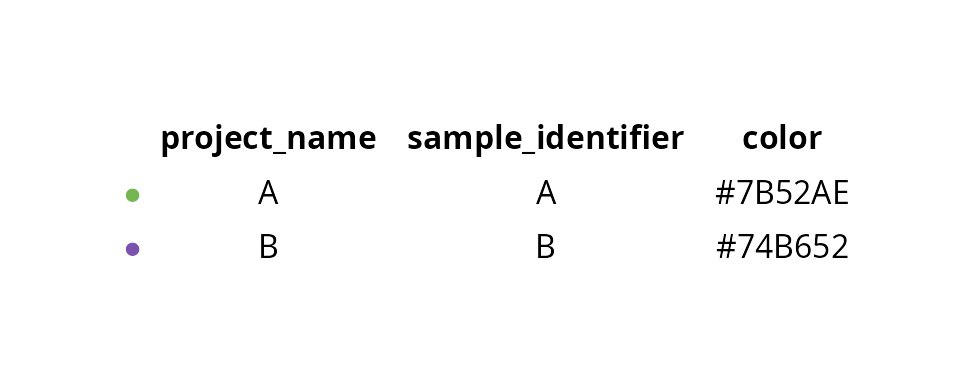
We set main parameters:
n_threads = 10L # Rtsne::Rtsne optionMake combined dataset
Individual datasets
For each sample, we:
- load individual dataset
- look at cell annotation
We load individual datasets:
sobj_list = lapply(sample_info$project_name, FUN = function(one_project_name) {
  sobj = readRDS(paste0(data_path, one_project_name, "_sobj_filtered.rds"))
  return(sobj)
})
names(sobj_list) = sample_info$project_name

lapply(sobj_list, FUN = dim) %>%
  do.call(rbind, .) %>%
  rbind(., colSums(.)) %>%
  `colnames<-`(c("Nb genes", "Nb cells"))
## Nb genes Nb cells
## A 28000 563
## B 28000 545
## 56000 1108We represent cells in the tSNE:
name2D = "RNA_pca_20_tsne"We look at cell type annotation for each dataset:
plot_list = lapply(sobj_list, FUN = function(sobj) {
  mytitle = as.character(unique(sobj@project.name))
  mysubtitle = ncol(sobj)

  p = Seurat::DimPlot(sobj, group.by = "cell_type",
                      reduction = name2D) +
    ggplot2::scale_color_manual(values = color_markers,
                                breaks = names(color_markers),
                                name = "Cell Type") +
    ggplot2::labs(title = mytitle,
                  subtitle = paste0(mysubtitle, " cells")) +
    ggplot2::theme(aspect.ratio = 1,
                   plot.title = element_text(hjust = 0.5),
                   plot.subtitle = element_text(hjust = 0.5)) +
    Seurat::NoAxes()

  return(p)
})

plot_list[[length(plot_list) + 1]] = patchwork::guide_area()

patchwork::wrap_plots(plot_list, nrow = 1) +
  patchwork::plot_layout(guides = "collect") &
  ggplot2::theme(legend.position = "right")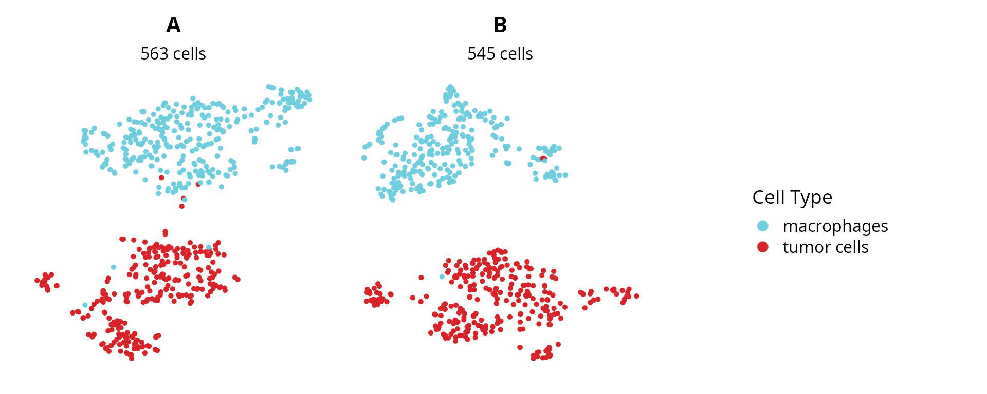
and clustering:
plot_list = lapply(sobj_list, FUN = function(sobj) {
  mytitle = as.character(unique(sobj@project.name))
  mysubtitle = ncol(sobj)

  p = Seurat::DimPlot(sobj, group.by = "seurat_clusters",
                      reduction = name2D, label = TRUE) +
    ggplot2::labs(title = mytitle,
                  subtitle = paste0(mysubtitle, " cells")) +
    ggplot2::theme(aspect.ratio = 1,
                   plot.title = element_text(hjust = 0.5),
                   plot.subtitle = element_text(hjust = 0.5)) +
    Seurat::NoAxes() + Seurat::NoLegend()

  return(p)
})

patchwork::wrap_plots(plot_list, nrow = 1)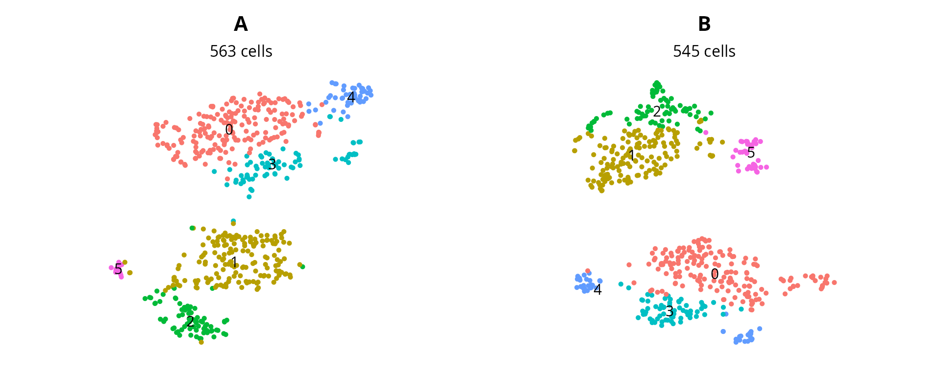
Combined dataset
We combine all datasets:
sobj = base::merge(sobj_list[[1]],
                   y = sobj_list[c(2:length(sobj_list))],
                   add.cell.ids = names(sobj_list))
sobj
## An object of class Seurat
## 28000 features across 1108 samples within 1 assay
## Active assay: RNA (28000 features, 3000 variable features)
## 6 layers present: counts.A, counts.B, data.A, scale.data.A, data.B, scale.data.BWe merge the layers:
sobj = SeuratObject::JoinLayers(sobj, layers = "counts")
sobj = SeuratObject::JoinLayers(sobj, layers = "data")
sobj = SeuratObject::JoinLayers(sobj, layers = "scale.data")

sobj
## An object of class Seurat
## 28000 features across 1108 samples within 1 assay
## Active assay: RNA (28000 features, 3000 variable features)
## 3 layers present: scale.data, data, countsWe add again the correspondence between gene names and gene ID. Since all datasets have been aligned using the same transcriptome, we take the correspondence from one individual dataset.
sobj@assays$RNA@meta.data = sobj_list[[1]]@assays$RNA@meta.data[, c("Ensembl_ID", "gene_name")]

head(sobj@assays$RNA@meta.data)
## Ensembl_ID gene_name
## Xkr4 ENSMUSG00000051951 Xkr4
## Gm1992 ENSMUSG00000089699 Gm1992
## Gm37381 ENSMUSG00000102343 Gm37381
## Rp1 ENSMUSG00000025900 Rp1
## Rp1.1 ENSMUSG00000109048 Rp1
## Sox17 ENSMUSG00000025902 Sox17We remove the list of objects:
rm(sobj_list)What is are the cells metadata ?
summary(sobj@meta.data)## orig.ident nCount_RNA nFeature_RNA log_nCount_RNA
## Length:1108 Min. : 873 Min. : 600 Min. : 6.772
## Class :character 1st Qu.: 2857 1st Qu.:1290 1st Qu.: 7.958
## Mode :character Median : 6245 Median :2346 Median : 8.740
## Mean : 7428 Mean :2292 Mean : 8.630
## 3rd Qu.:10746 3rd Qu.:3070 3rd Qu.: 9.282
## Max. :37168 Max. :6042 Max. :10.523
## Seurat.Phase cyclone.Phase RNA_snn_res.0.5 seurat_clusters
## Length:1108 Length:1108 Length:1108 Length:1108
## Class :character Class :character Class :character Class :character
## Mode :character Mode :character Mode :character Mode :character
##
##
##
## percent.mt percent.rb score_macrophages score_tumor_cells
## Min. : 0.000 Min. : 0.1894 Min. :-1.2490 Min. :-0.9281
## 1st Qu.: 3.036 1st Qu.: 2.8973 1st Qu.:-0.8256 1st Qu.:-0.8095
## Median : 4.721 Median : 6.9742 Median :-0.2001 Median :-0.5249
## Mean : 7.192 Mean : 7.0765 Mean :-0.1171 Mean :-0.1145
## 3rd Qu.:10.797 3rd Qu.:10.2290 3rd Qu.: 0.6220 3rd Qu.: 0.6046
## Max. :19.959 Max. :19.9397 Max. : 1.6646 Max. : 2.2151
## cell_type
## Length:1108
## Class :character
## Mode :character
##
##
## Processing
We remove genes that are expressed in less than 5 cells:
sobj = aquarius::filter_features(sobj, min_cells = 5)
sobj
## An object of class Seurat
## 13774 features across 1108 samples within 1 assay
## Active assay: RNA (13774 features, 0 variable features)
## 3 layers present: scale.data, data, countsMetadata
How many cells by sample ?
table(sobj$orig.ident)##
## A B
## 563 545We represent this information as a barplot:
aquarius::plot_barplot(df = table(sobj$orig.ident,
                                  sobj$cell_type) %>%
                         as.data.frame.table() %>%
                         `colnames<-`(c("Sample", "Cell Type", "Number")),
                       x = "Sample", y = "Number", fill = "Cell Type",
                       position = position_fill()) +
  ggplot2::scale_fill_manual(values = unlist(color_markers),
                             breaks = names(color_markers),
                             name = "Cell Type")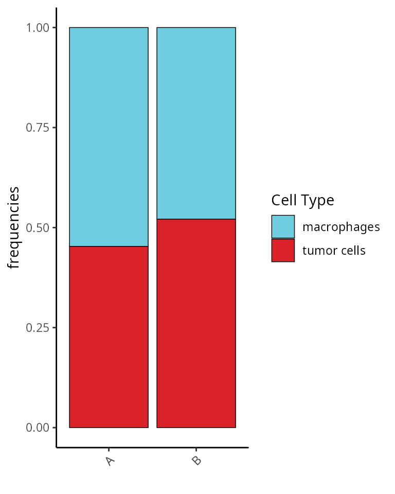
This is the same barplot with another position:
aquarius::plot_barplot(df = table(sobj$orig.ident,
                                  sobj$cell_type) %>%
                         as.data.frame.table() %>%
                         `colnames<-`(c("Sample", "Cell Type", "Number")),
                       x = "Sample", y = "Number", fill = "Cell Type",
                       position = position_stack()) +
  ggplot2::scale_fill_manual(values = unlist(color_markers),
                             breaks = names(color_markers),
                             name = "Cell Type")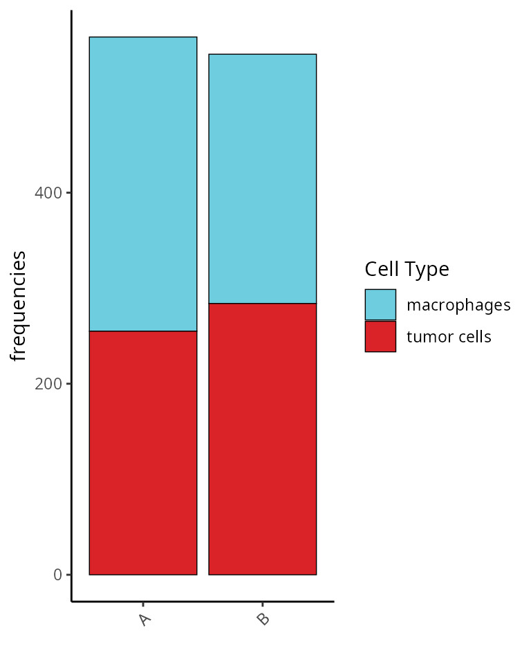
Projection
We normalize the count matrix for remaining cells and select highly variable features:
sobj = Seurat::NormalizeData(sobj,
                             normalization.method = "LogNormalize")
sobj = Seurat::FindVariableFeatures(sobj, nfeatures = 2000)
sobj = Seurat::ScaleData(sobj)

sobj
## An object of class Seurat
## 13774 features across 1108 samples within 1 assay
## Active assay: RNA (13774 features, 2000 variable features)
## 3 layers present: scale.data, data, countsWe perform a PCA:
sobj = Seurat::RunPCA(sobj,
                      assay = "RNA",
                      reduction.name = "RNA_pca",
                      npcs = 100,
                      seed.use = 1337L)
sobj
## An object of class Seurat
## 13774 features across 1108 samples within 1 assay
## Active assay: RNA (13774 features, 2000 variable features)
## 3 layers present: scale.data, data, counts
## 1 dimensional reduction calculated: RNA_pcaWe choose the number of dimensions such that they summarize 60 % of the variability:
stdev = sobj@reductions[["RNA_pca"]]@stdev
stdev_prop = cumsum(stdev)/sum(stdev)
ndims = which(stdev_prop > 0.60)[1]
ndims
## [1] 48We can visualize this on the elbow plot:
elbow_p = Seurat::ElbowPlot(sobj, ndims = 100, reduction = "RNA_pca") +
  ggplot2::geom_point(x = ndims, y = stdev[ndims], col = "red")
x_text = ggplot_build(elbow_p)$layout$panel_params[[1]]$x$get_labels() %>% as.numeric()
elbow_p = elbow_p +
  ggplot2::scale_x_continuous(breaks = sort(c(x_text, ndims)), limits = c(0, 100))
x_color = ifelse(ggplot_build(elbow_p)$layout$panel_params[[1]]$x$get_labels() %>%
                   as.numeric() %>% round(., 2) == round(ndims, 2), "red", "black")
elbow_p = elbow_p +
  ggplot2::theme_classic() +
  ggplot2::theme(axis.text.x = element_text(color = x_color))

elbow_p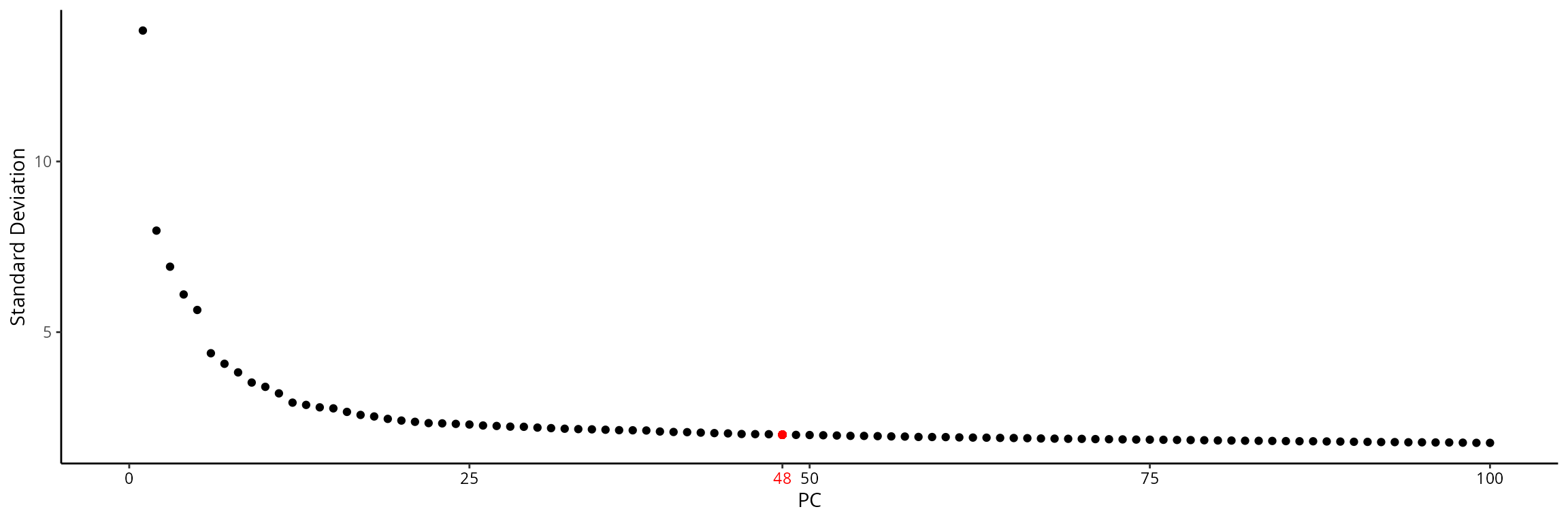
We generate a tSNE and a UMAP with 48 principal components:
sobj = Seurat::RunTSNE(sobj,
                       reduction = "RNA_pca",
                       dims = 1:ndims,
                       seed.use = 1337L,
                       num_threads = n_threads, # Rtsne::Rtsne option
                       reduction.name = paste0("RNA_pca_", ndims, "_tsne"))

sobj = Seurat::RunUMAP(sobj,
                       reduction = "RNA_pca",
                       dims = 1:ndims,
                       seed.use = 1337L,
                       reduction.name = paste0("RNA_pca_", ndims, "_umap"))
(Time to run: 5.29 s)
We can visualize the two representations:
tsne = Seurat::DimPlot(sobj, group.by = "orig.ident",
                       reduction = paste0("RNA_pca_", ndims, "_tsne")) +
  ggplot2::scale_color_manual(values = sample_info$color,
                              breaks = sample_info$project_name) +
  Seurat::NoAxes() + ggplot2::ggtitle("PCA - tSNE") +
  ggplot2::theme(aspect.ratio = 1,
                 plot.title = element_text(hjust = 0.5),
                 legend.position = "none")

umap = Seurat::DimPlot(sobj, group.by = "orig.ident",
                       reduction = paste0("RNA_pca_", ndims, "_umap")) +
  ggplot2::scale_color_manual(values = sample_info$color,
                              breaks = sample_info$project_name) +
  Seurat::NoAxes() + ggplot2::ggtitle("PCA - UMAP") +
  ggplot2::theme(aspect.ratio = 1,
                 plot.title = element_text(hjust = 0.5))

tsne | umap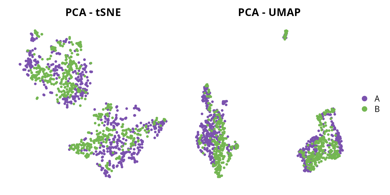
Batch-effect correction
We remove sample specific effect on the pca using
harmony:
`%||%` = function(lhs, rhs) {
if (!is.null(x = lhs)) {
return(lhs)
} else {
return(rhs)
}
}
set.seed(1337L)
sobj = harmony::RunHarmony(object = sobj,
group.by.vars = "orig.ident",
plot_convergence = TRUE,
reduction = "RNA_pca",
assay.use = "RNA",
reduction.save = "harmony",
max.iter.harmony = 50,
project.dim = FALSE)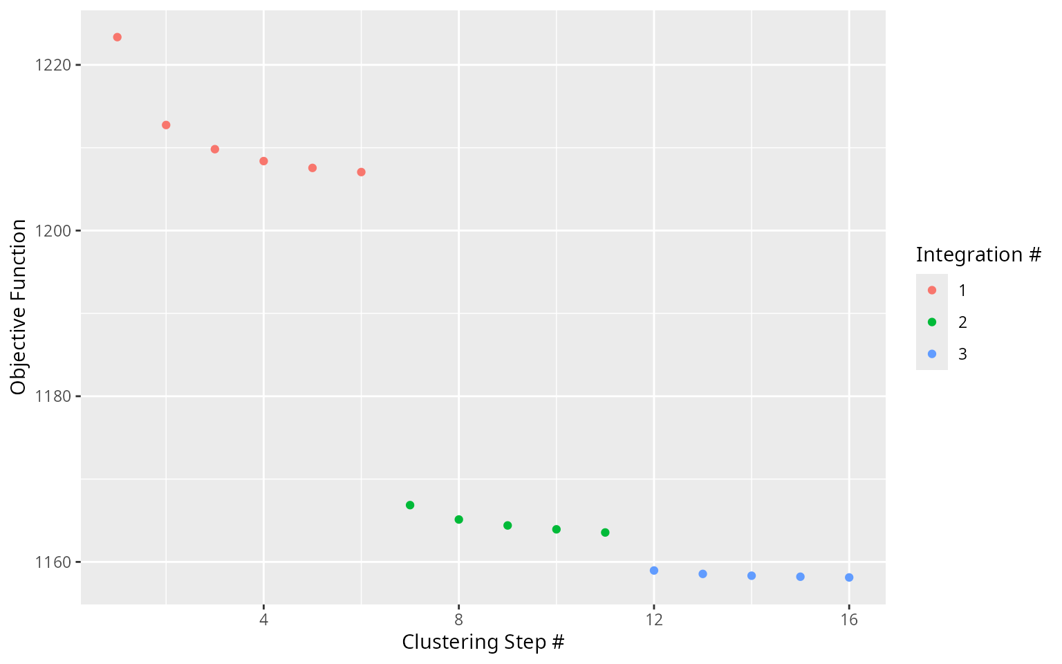 (Time
to run: 0.83 s)
(Time
to run: 0.83 s)
From this batch-effect removed projection, we generate a tSNE and a UMAP.
sobj = Seurat::RunUMAP(sobj,
                       seed.use = 1337L,
                       dims = 1:ndims,
                       reduction = "harmony",
                       reduction.name = paste0("harmony_", ndims, "_umap"),
                       reduction.key = paste0("harmony_", ndims, "umap_"))

sobj = Seurat::RunTSNE(sobj,
                       dims = 1:ndims,
                       seed.use = 1337L,
                       num_threads = n_threads, # Rtsne::Rtsne option
                       reduction = "harmony",
                       reduction.name = paste0("harmony_", ndims, "_tsne"),
                       reduction.key = paste0("harmony", ndims, "tsne_"))
(Time to run: 5.49 s)
We visualize the corrected projections:
tsne = Seurat::DimPlot(sobj, group.by = "orig.ident",
                       reduction = paste0("harmony_", ndims, "_tsne")) +
  ggplot2::scale_color_manual(values = sample_info$color,
                              breaks = sample_info$project_name) +
  Seurat::NoAxes() + ggplot2::ggtitle("PCA - harmony - tSNE") +
  ggplot2::theme(aspect.ratio = 1,
                 plot.title = element_text(hjust = 0.5),
                 legend.position = "none")

umap = Seurat::DimPlot(sobj, group.by = "orig.ident",
                       reduction = paste0("harmony_", ndims, "_umap")) +
  ggplot2::scale_color_manual(values = sample_info$color,
                              breaks = sample_info$project_name) +
  Seurat::NoAxes() + ggplot2::ggtitle("PCA - harmony - UMAP") +
  ggplot2::theme(aspect.ratio = 1,
                 plot.title = element_text(hjust = 0.5))

tsne | umap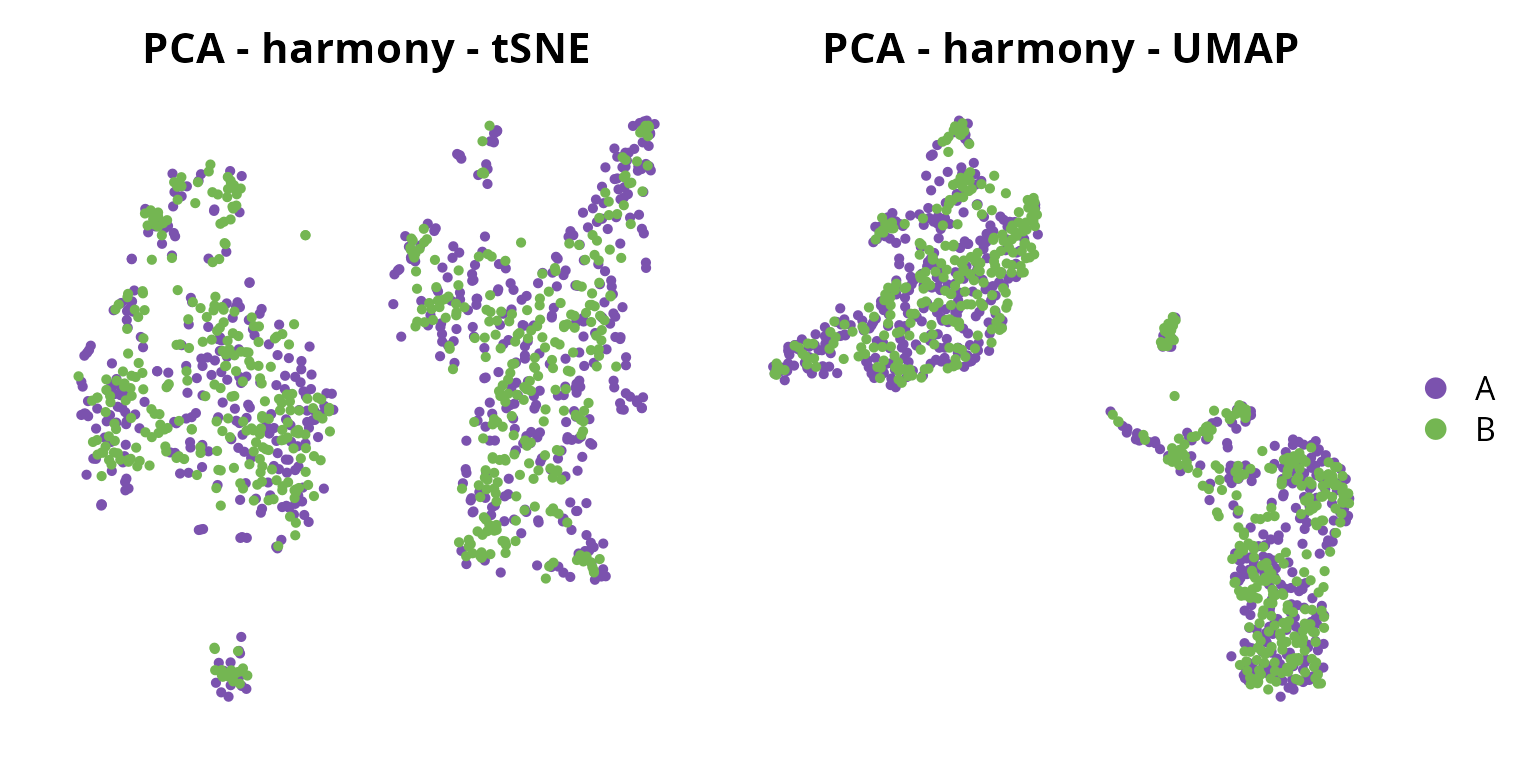
We will keep the tSNE from harmony:
reduction = "harmony"
name2D = paste0("harmony_", ndims, "_tsne")
Clustering
We generate a clustering:
sobj = Seurat::FindNeighbors(sobj, reduction = reduction, dims = 1:ndims)
sobj = Seurat::FindClusters(sobj, resolution = 0.5)
## Modularity Optimizer version 1.3.0 by Ludo Waltman and Nees Jan van Eck
##
## Number of nodes: 1108
## Number of edges: 44757
##
## Running Louvain algorithm...
## Maximum modularity in 10 random starts: 0.8318
## Number of communities: 8
## Elapsed time: 0 seconds
clusters_plot = Seurat::DimPlot(sobj, reduction = name2D, label = TRUE) +
  Seurat::NoAxes() + Seurat::NoLegend() +
  ggplot2::labs(title = "Clusters ID") +
  ggplot2::theme(aspect.ratio = 1,
                 plot.title = element_text(hjust = 0.5))
clusters_plot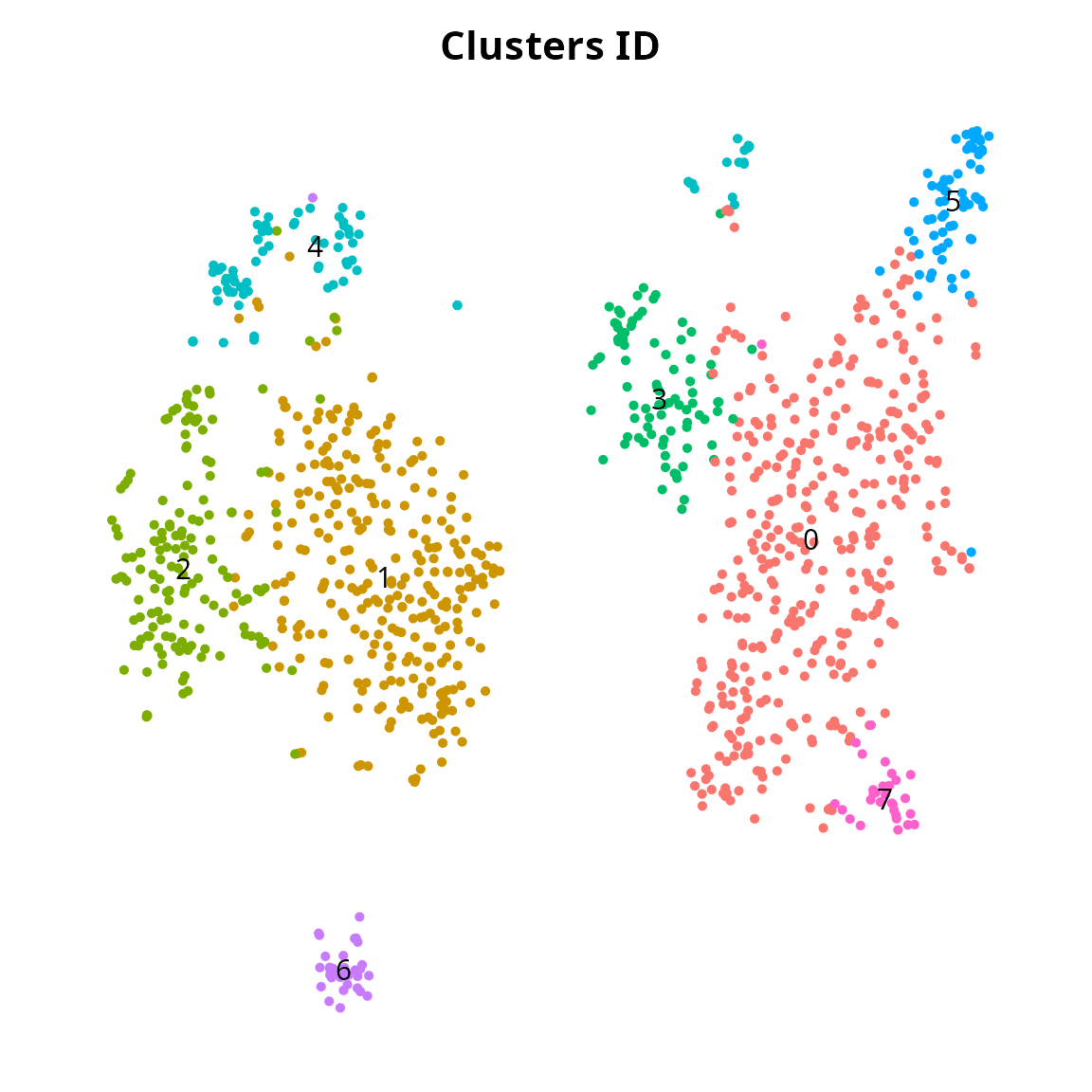
Visualization
We represent the 4 quality metrics:
plot_list = Seurat::FeaturePlot(sobj, reduction = name2D,
                                combine = FALSE, pt.size = 0.25,
                                features = c("percent.mt", "percent.rb", "log_nCount_RNA", "nFeature_RNA"))
plot_list = lapply(plot_list, FUN = function(one_plot) {
  one_plot +
    Seurat::NoAxes() +
    ggplot2::scale_color_gradientn(colors = aquarius::palette_GrOrBl) +
    ggplot2::theme(aspect.ratio = 1)
})

patchwork::wrap_plots(plot_list, nrow = 1)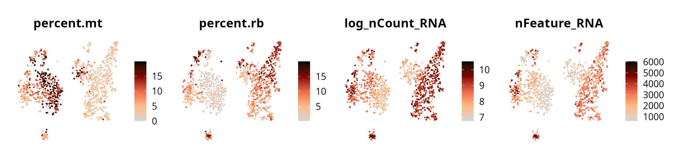
Clusters
We can represent clusters, split by sample of origin:
plot_list = aquarius::plot_split_dimred(
  sobj,
  reduction = name2D,
  split_by = "orig.ident",
  group_by = "seurat_clusters",
  split_color = setNames(sample_info$color,
                         nm = sample_info$project_name),
  bg_pt_size = 1, main_pt_size = 1)

plot_list[[length(plot_list) + 1]] = clusters_plot +
  ggplot2::labs(title = "Cluster ID") &
  ggplot2::theme(plot.title = element_text(hjust = 0.5, size = 15))

patchwork::wrap_plots(plot_list, nrow = 1) &
  Seurat::NoLegend()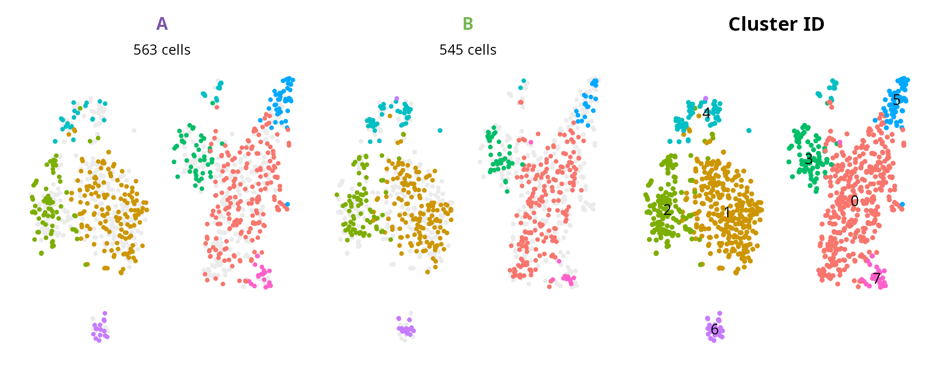
We make a heatmap to compare the representativness of cells for each sample, within each cluster:
aquarius::plot_prop_heatmap(df = sobj@meta.data[, c("orig.ident", "seurat_clusters")],
                            prop_margin = 1,
                            row_title = "Sample",
                            column_title = "Cluster ID")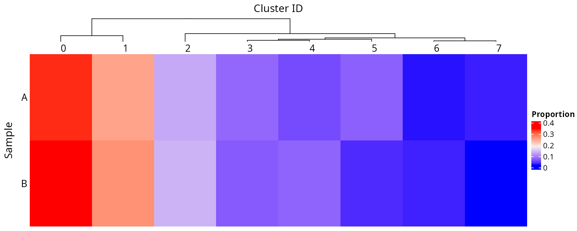
Cell type
We visualize cell type:
plot_list = lapply((c(paste0("RNA_pca_", ndims, "_tsne"),
                      paste0("RNA_pca_", ndims, "_umap"),
                      paste0("harmony_", ndims, "_tsne"),
                      paste0("harmony_", ndims, "_umap"))),
                   FUN = function(one_red) {
                     Seurat::DimPlot(sobj, group.by = "cell_type",
                                     reduction = one_red,
                                     cols = color_markers) +
                       Seurat::NoAxes() + ggplot2::ggtitle(one_red) +
                       ggplot2::theme(aspect.ratio = 1,
                                      plot.title = element_text(hjust = 0.5))
                   })

patchwork::wrap_plots(plot_list, nrow = 2) +
  patchwork::plot_layout(guides = "collect")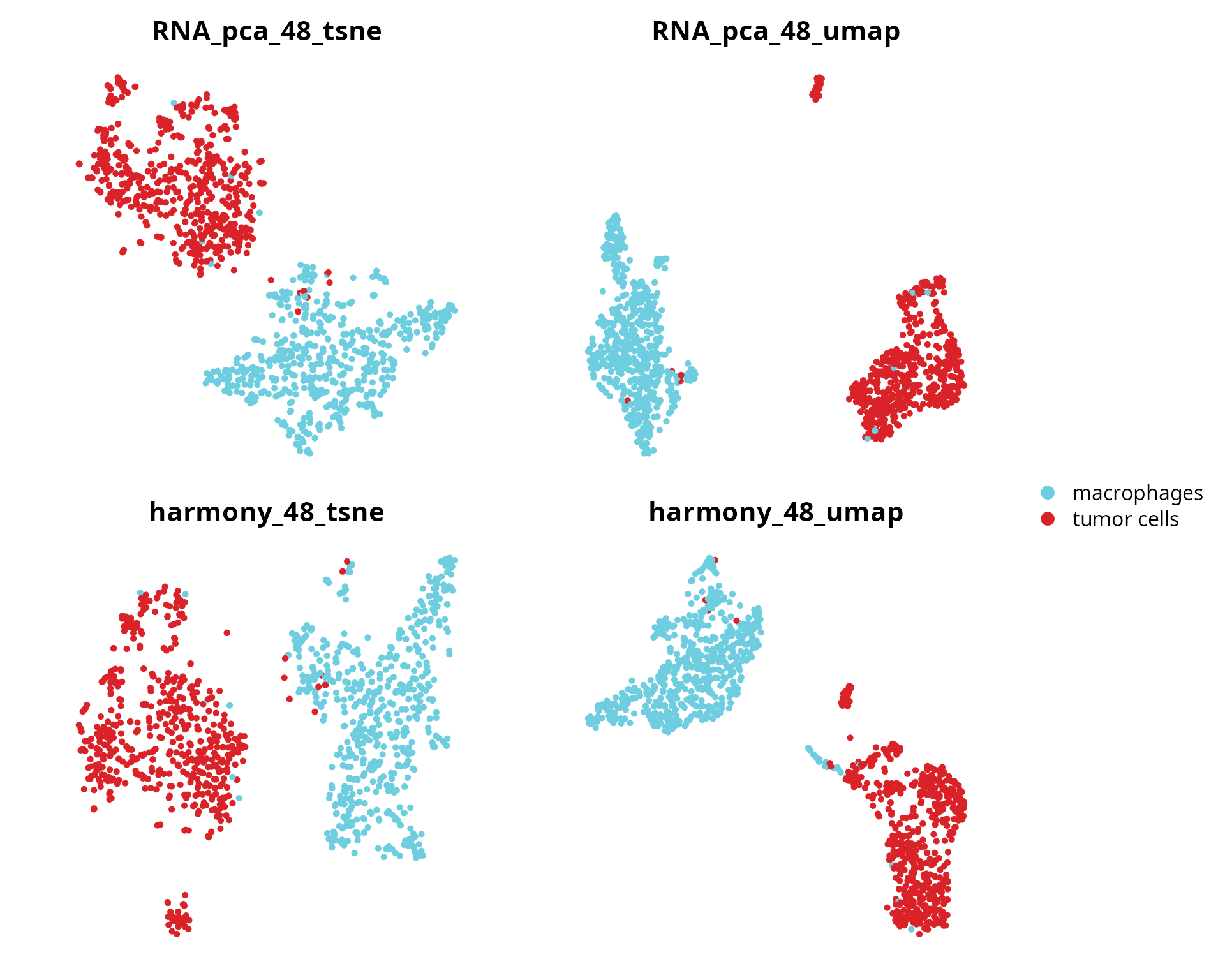
We make a representation split by origin to show cell types:
plot_list = aquarius::plot_split_dimred(sobj,
                                        reduction = name2D,
                                        split_by = "orig.ident",
                                        split_color = setNames(sample_info$color,
                                                               nm = sample_info$project_name),
                                        group_by = "cell_type",
                                        group_color = color_markers,
                                        main_pt_size = 1,
                                        bg_pt_size = 1)

plot_list[[length(plot_list) + 1]] = patchwork::guide_area()

patchwork::wrap_plots(plot_list, nrow = 1) +
  patchwork::plot_layout(guides = "collect") &
  ggplot2::theme(legend.position = "right")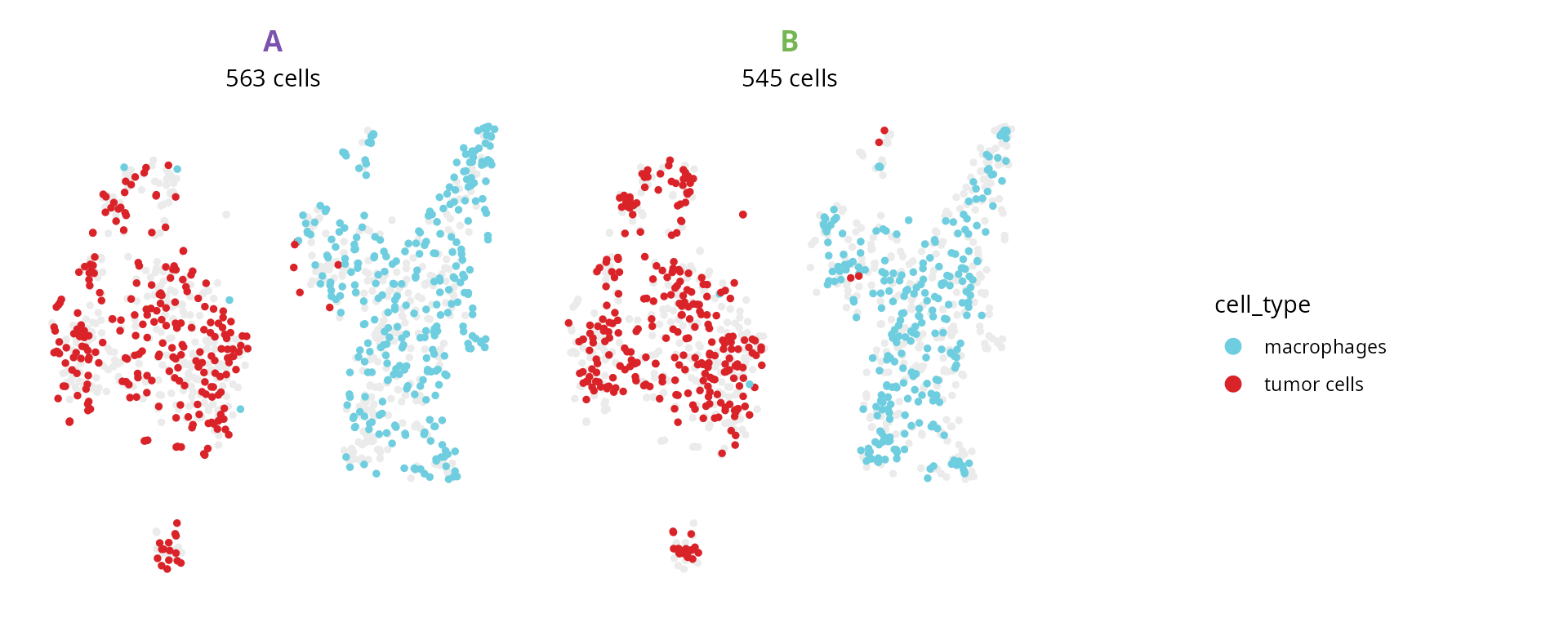
Cell cycle
We visualize cell cycle annotation, and Birc5 and Top2a expression levels:
plot_list = list()

# Seurat
plot_list[[1]] = Seurat::DimPlot(sobj, group.by = "Seurat.Phase",
                                 reduction = name2D) +
  Seurat::NoAxes() + ggplot2::labs(title = "Seurat annotation") +
  ggplot2::theme(aspect.ratio = 1,
                 plot.title = element_text(hjust = 0.5))

# cyclone
plot_list[[2]] = Seurat::DimPlot(sobj, group.by = "cyclone.Phase",
                                 reduction = name2D) +
  Seurat::NoAxes() + ggplot2::labs(title = "cyclone annotation") +
  ggplot2::theme(aspect.ratio = 1,
                 plot.title = element_text(hjust = 0.5))

# BIRC5
plot_list[[3]] = Seurat::FeaturePlot(sobj, features = "Birc5",
                                     reduction = name2D) +
  ggplot2::scale_color_gradientn(colors = aquarius::palette_GrOrBl) +
  Seurat::NoAxes() +
  ggplot2::theme(aspect.ratio = 1,
                 plot.title = element_text(hjust = 0.5))

# TOP2A
plot_list[[4]] = Seurat::FeaturePlot(sobj, features = "Top2a",
                                     reduction = name2D) +
  ggplot2::scale_color_gradientn(colors = aquarius::palette_GrOrBl) +
  Seurat::NoAxes() +
  ggplot2::theme(aspect.ratio = 1,
                 plot.title = element_text(hjust = 0.5))

patchwork::wrap_plots(plot_list, ncol = 2)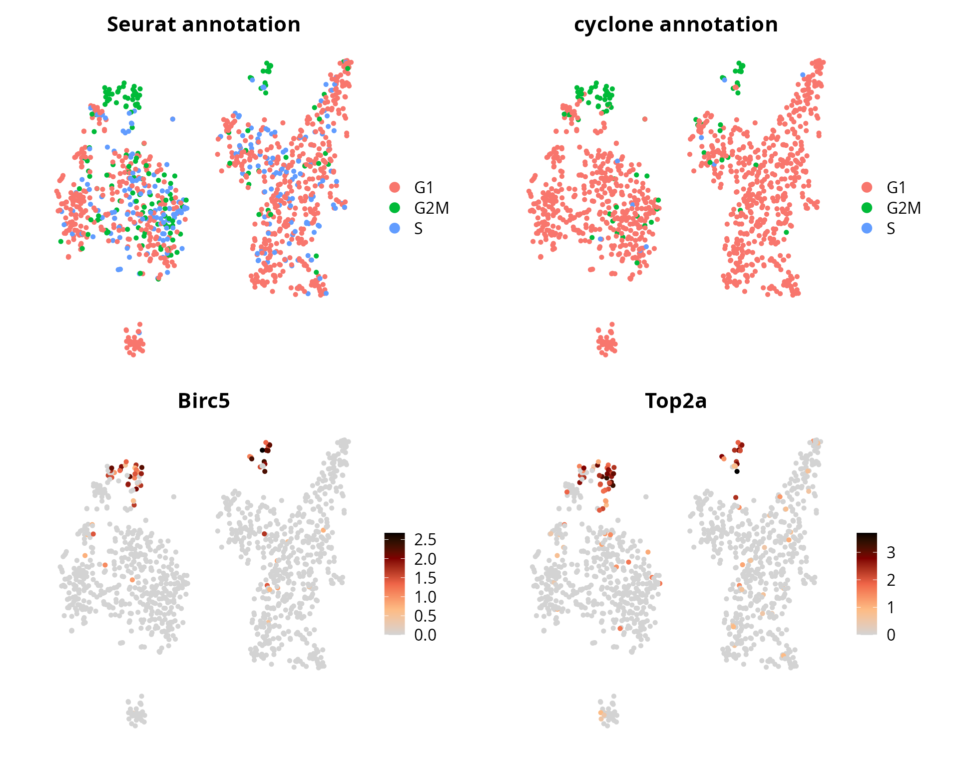
R Session
show
## R version 4.4.3 (2025-02-28)
## Platform: x86_64-pc-linux-gnu
## Running under: Ubuntu 24.10
##
## Matrix products: default
## BLAS:   /usr/lib/x86_64-linux-gnu/blas/libblas.so.3.12.0
## LAPACK: /usr/lib/x86_64-linux-gnu/lapack/liblapack.so.3.12.0
##
## locale:
##  [1] LC_CTYPE=en_US.UTF-8       LC_NUMERIC=C
##  [3] LC_TIME=fr_FR.UTF-8        LC_COLLATE=en_US.UTF-8
##  [5] LC_MONETARY=fr_FR.UTF-8    LC_MESSAGES=en_US.UTF-8
##  [7] LC_PAPER=fr_FR.UTF-8       LC_NAME=C
##  [9] LC_ADDRESS=C               LC_TELEPHONE=C
## [11] LC_MEASUREMENT=fr_FR.UTF-8 LC_IDENTIFICATION=C
##
## time zone: Europe/Paris
## tzcode source: system (glibc)
##
## attached base packages:
## [1] stats     graphics  grDevices utils     datasets  methods   base
##
## other attached packages:
## [1] future_1.40.0   ggplot2_3.5.2   patchwork_1.3.0 dplyr_1.1.4
##
## loaded via a namespace (and not attached):
##   [1] RColorBrewer_1.1-3          jsonlite_2.0.0
##   [3] shape_1.4.6.1               magrittr_2.0.3
##   [5] spatstat.utils_3.1-3        farver_2.1.2
##   [7] rmarkdown_2.29              zlibbioc_1.52.0
##   [9] GlobalOptions_0.1.2         fs_1.6.6
##  [11] ragg_1.4.0                  vctrs_0.6.5
##  [13] ROCR_1.0-11                 Cairo_1.6-2
##  [15] spatstat.explore_3.4-2      S4Arrays_1.6.0
##  [17] htmltools_0.5.8.1           SparseArray_1.6.2
##  [19] sass_0.4.10                 sctransform_0.4.2
##  [21] parallelly_1.43.0           KernSmooth_2.23-26
##  [23] bslib_0.9.0                 htmlwidgets_1.6.4
##  [25] desc_1.4.3                  ica_1.0-3
##  [27] plyr_1.8.9                  plotly_4.10.4
##  [29] zoo_1.8-14                  cachem_1.1.0
##  [31] igraph_2.1.4                mime_0.13
##  [33] lifecycle_1.0.4             iterators_1.0.14
##  [35] pkgconfig_2.0.3             Matrix_1.7-3
##  [37] R6_2.6.1                    fastmap_1.2.0
##  [39] GenomeInfoDbData_1.2.13     MatrixGenerics_1.18.1
##  [41] fitdistrplus_1.2-2          shiny_1.10.0
##  [43] clue_0.3-66                 digest_0.6.37
##  [45] colorspace_2.1-1            S4Vectors_0.44.0
##  [47] Seurat_5.3.0                tensor_1.5
##  [49] RSpectra_0.16-2             irlba_2.3.5.1
##  [51] GenomicRanges_1.58.0        textshaping_1.0.1
##  [53] labeling_0.4.3              progressr_0.15.1
##  [55] spatstat.sparse_3.1-0       httr_1.4.7
##  [57] polyclip_1.10-7             abind_1.4-8
##  [59] compiler_4.4.3              withr_3.0.2
##  [61] doParallel_1.0.17           BiocParallel_1.40.2
##  [63] fastDummies_1.7.5           MASS_7.3-65
##  [65] DelayedArray_0.32.0         rjson_0.2.23
##  [67] tools_4.4.3                 lmtest_0.9-40
##  [69] httpuv_1.6.16               future.apply_1.11.3
##  [71] goftest_1.2-3               glue_1.8.0
##  [73] nlme_3.1-168                promises_1.3.2
##  [75] grid_4.4.3                  Rtsne_0.17
##  [77] cluster_2.1.8.1             reshape2_1.4.4
##  [79] generics_0.1.3              gtable_0.3.6
##  [81] spatstat.data_3.1-6         ggpattern_1.1.4
##  [83] tidyr_1.3.1                 data.table_1.17.0
##  [85] XVector_0.46.0              sp_2.2-0
##  [87] BiocGenerics_0.52.0         spatstat.geom_3.3-6
##  [89] RcppAnnoy_0.0.22            ggrepel_0.9.6
##  [91] RANN_2.6.2                  foreach_1.5.2
##  [93] pillar_1.10.2               stringr_1.5.1
##  [95] spam_2.11-1                 RcppHNSW_0.6.0
##  [97] later_1.4.2                 circlize_0.4.16
##  [99] splines_4.4.3               lattice_0.22-6
## [101] survival_3.8-3              deldir_2.0-4
## [103] aquarius_1.0.0              tidyselect_1.2.1
## [105] SingleCellExperiment_1.28.1 ComplexHeatmap_2.23.1
## [107] miniUI_0.1.2                pbapply_1.7-2
## [109] knitr_1.50                  gridExtra_2.3
## [111] IRanges_2.40.1              SummarizedExperiment_1.36.0
## [113] scattermore_1.2             RhpcBLASctl_0.23-42
## [115] stats4_4.4.3                xfun_0.52
## [117] Biobase_2.66.0              matrixStats_1.5.0
## [119] UCSC.utils_1.2.0            stringi_1.8.7
## [121] lazyeval_0.2.2              yaml_2.3.10
## [123] evaluate_1.0.3              codetools_0.2-20
## [125] tibble_3.2.1                cli_3.6.5
## [127] uwot_0.2.3                  xtable_1.8-4
## [129] reticulate_1.42.0           systemfonts_1.2.3
## [131] jquerylib_0.1.4             harmony_1.2.3
## [133] GenomeInfoDb_1.42.3         Rcpp_1.0.14
## [135] spatstat.random_3.3-3       globals_0.17.0
## [137] png_0.1-8                   spatstat.univar_3.1-2
## [139] parallel_4.4.3              pkgdown_2.1.2
## [141] dotCall64_1.2               listenv_0.9.1
## [143] viridisLite_0.4.2           scales_1.4.0
## [145] ggridges_0.5.6              SeuratObject_5.1.0
## [147] purrr_1.0.4                 crayon_1.5.3
## [149] GetoptLong_1.0.5            rlang_1.1.6
## [151] cowplot_1.1.3